
Step Through Scatter Plot Construction
Loading the math board and drawing, please wait…
In collections
Statistics Step Through Applets
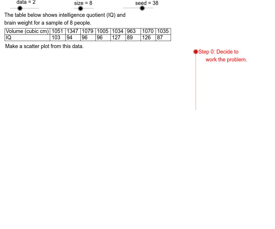
This example demonstrates how to construct scatter diagrams by varying data types, sample sizes, and subsets. It involves core math concepts like statistical analysis, standard deviation, and function graphing (hyperbolas, trigonometric functions). Construction highlights include commands like Element, Sequence, Max, Min, If, Segment, Text, and objects such as CW, DtStr, GL, GR, GB. Ideal for high school students and math enthusiasts exploring statistics, calculus, and coordinate geometry.
GeoGebra Commands & Parameters
Element(SmpRtSq, Mod[seed, 6] + 1) → SmpRtElement(DtXSq, data) → DtX1Sequence(Element[DtX1, Mod[Strt + (k * SmpRt), 15] + 1], k, 0, size - 1) → DtX2Max(DtX2) → XMaxMin(DtX2) → XMinIf((5 * LBSX) ≤ UBSX, (5 * LBSX), If[(2 * LBSX) ≤ UBSX, (2 * LBSX), LBSX]) → XSclElement(DtYSq, data) → DtY1Sequence(Element[DtY1, Mod[Strt + (k * SmpRt), 15] + 1], k, 0, size - 1) → DtY2Min(DtY2) → YMinMax(DtY2) → YMaxSegment(Origin, HAE) → HAxSegment(Origin, VAE) → VAxIf((5 * LBSY) ≤ UBSY, (5 * LBSY), If[(2 * LBSY) ≤ UBSY, (2 * LBSY), LBSY]) → YSclSequence(AdpX(Element[DtX2, k]), k, 1, size) → PltXSequence(AdpY(Element[DtY2, k]), k, 1, size) → PltYSequence((Element[PltX, k], Element[PltY, k]), k, 1, size) → DtPntsSegment(UL, UR) → TbTpSegment(ML, MR) → TBMdSegment(LL, LR) → TbBtSegment(LL, UL) → LeftSegment(LM, UM) → DatLeftSequence(Segment[(AdpX(k), GB - 0.5), (AdpX(k), GB + 0.5)], k, XAxMin, XAxMax, XScl) → XTcSequence(Text[k, (AdpX(k) - 1, GB - 2.5)], k, XAxMin, XAxMax, XScl) → XLbsSequence(Segment[(GL - 0.5, AdpY(k)), (GL + 0.5, AdpY(k))], k, YAxMn, YAxMx, YScl) → YTcElement(XVSq1, data) → XAxLbElement(YVSq1, data) → YAxLbText(Element[XVSq1, data], (DtStr - 11.65, DtHgt - 1.9)) → XVTx1Text(Element[YVSq1, data], (DtStr - 11.65, DtHgt - 4.4)) → YVTx1Sequence(Segment[(DtStr + 6.2 + (k * CW), DtHgt), (DtStr + 6.2 + (k * CW), DtHgt - 5)], k, 1, size) → DvLnSequence(Text[Element[DtY2, k], (DtStr + 0.7 + (CW * k), DtHgt - 4.4)], k, 1, size) → YDtTxtSequence(Text[Element[DtX2, k], (DtStr + 0.7 + (CW * k), DtHgt - 1.9)], k, 1, size) → XDtTxtElement(DDSq, data) → DDElement(XVSq2, data) → XVTx2Element(YVSq2, data) → YVTx2Sequence(Text[k, ((-3), AdpY(k) - 0.35)], k, YAxMn, YAxMx, YScl) → YLbsElement(TtlSq, data) → Ttl
AI Drawing Prompt Reference
Create a scatter plot with X-axis and Y-axis ranging from XMin to XMax and YMin to YMax respectively. Mark the axes with ticks and labels, where the X-axis label is XAxLb and the Y-axis label is YAxLb. The scatter plot consists of points generated from DtX2 and DtY2, with coordinates AdpX and AdpY. Above the plot, there is a title Ttl, and vertical and horizontal dividing lines on the left and right sides. The X-axis and Y-axis have tick lines XTc and YTc, and corresponding tick labels XLbs and YLbs.
The prompt above was compiled from the original drawing commands and is for reference only.