
Step Through Histogram Construction
Loading the math board and drawing, please wait…
In collections
Statistics Step Through Applets
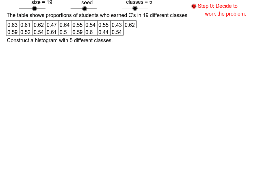
This example demonstrates the step-by-step process of constructing a histogram. It involves core mathematical concepts like data binning, frequency counting, and adjusting sample size. GeoGebra commands and objects such as Mod, Sequence, Min, Max, If, Sort, CountIf, Append, Element, Segment, Text, VerticalText, GrHt, GrTp, GrBt, GrLf, classes, seed, ACDT, size, L0, L1, Mn1, MxX1, UB, LB, CWC4, CWC3, CWC2, CWC1, CW0, MxX2, FrqSq, MxFq1, VSc1, MxFq2, GrWd, RtEnd, LfEnd, FDRt, FDTp, FDLf, LCLSq2, TbCW, TbLf, TbTp, TbCH, DTp, DLf, DWd, TbBt, sz1 are used in the construction. Suitable for high school mathematics teaching or statistics courses.
GeoGebra Commands & Parameters
Mod(seed, 3) → ACDTSequence(RandomPoisson[seed], k, 1, size) → L0Sequence((Element[L0, k] * 10^((-ACDT))), k, 1, size) → L1Min(L1) → Mn1Max(L1) → MxX1If(CWC1 ≤ UB, CWC1, If[CWC2 ≤ UB, CWC2, If[CWC3 ≤ UB, CWC3, CWC4]]) → CW0Sequence(CountIf[i ≤ x < i + CW0, L1], i, Mn1, MxX2 - CW0, CW0) → FrqSqMax(FrqSq) → MxFq1Sequence(k, k, Mn1, Mn1 + ((classes - 1) * CW0), CW0) → LCLSq2Sequence(Element[L1, k], k, 1, sz1) → L2Sequence(Element[LCLSq2, k], k, 1, classes - 1) → LCLSq1Sequence(k, k, Mn1, MxX1, 10^((-ACDT))) → DtDmSort(Intersection[DtDm, L1]) → DtRngCountIf(x < MxX1 + 1, DtRng) → RngCntMax(Sequence[If[floor((10^(k) * CW0)) / 10^(k) ≠ CW0, k + 1, 0], k, 0, 2]) → ACCWMax(ACDT, ACCW) → ACNwSequence(" to ", k, 1, classes) → ToSqAppend(Mn1, LCLSq1) → LCLCnSqElement(LCLSq2, 2) → LCL2Sequence(Element[L1, k], k, sz1 + 1, size) → L3Segment(TbML, TbMR) → tbmdSegment(TbLL, TbLR) → tbbtSegment(TbMR, TbUR) → tbrtSequence(CW1, k, 1, classes - 1) → CWSq1Append(" ", CWSq1) → CWSq2Sequence(UCL1 + (k * CW1), k, 0, classes - 1) → UCLSqAppend(UCL1, UCLSq) → UCLCnSqSequence(Sequence[" | ", k, 1, Element[FrqSq, j]], j, 1, classes) → TlySqSegment(TbUL, TbUR) → tbtpSequence(Segment[(TbLf + (k * TbCW), TbBt), (TbLf + (k * TbCW), TbTp)], k, 0, floor(size / 2)) → TbVrtSqText("The table shows the percent unemployed for " + size + " different cities.") → DD1Text("The table shows numbers of bird feeders sold in " + size + " different months.") → DD0Text("The table shows proportions of students who earned C's in " + size + " different classes.") → DD2Element(DDSq, ACDT + 1) → DDIf(ACDT ≟ 1, ".", "s.") → PLP1If(ACCW ≟ 1, "", "s") → PLN2If(ACNw ≟ 1, ".", "s.") → PLP3If(ACNw ≟ 1, "", "s") → PLN3Sequence(Text[Element[LCLSq2, k], (FDLf, FDTp - (0.07 * k))], k, 1, classes) → LCLTxSqIf(ACDT ≟ 1, "", "s") → PLN1Sequence(Text[Element[UCLSq, k], (FDLf + 8, FDTp - (FDRt * k))], k, 1, classes) → UCLTxSqSequence(Text[Element[ToSq, k], (FDLf + 4.5, FDTp - (0.07 * k))], k, 1, classes) → ToTxSqSequence(Text[Element[FrqSq, k], (FDLf + 15, FDTp - (FDRt * k))], k, 1, classes) → FrqTxSqText("Construct a histogram with " + classes + " different classes.") → PrbStmSegment(GrUL, GrLL) → gvaxSegment(GrLL, GrLR) → ghaxSequence(Text[(k * VSc1), (GrLf - 3, GrTp - GrHt - 0.025 + ((VSc1 * VSc2) * k))], k, 0, MxFq2 / VSc1) → VTcLbSequence(k, k, Mn1, Mn1 + (classes * CW0), CW0) → LCLSq3Sequence(adp2(Element[LCLSq3, k]), k, 1, classes + 1) → BESqSequence(Text[Element[LCLSq3, k], (Element[BESq, k] - 1.5, GrBt - 0.08)], k, 1, classes + 1) → HTcLbSequence(Segment[(Element[BESq, k], GrBt), (Element[BESq, k], GrBt - 0.02)], k, 1, classes + 1) → HTcsSequence(Segment[(GrLf - 0.5, GrBt + (k * VSc2)), (GrLf, GrBt + (k * VSc2))], k, 0, MxFq2) → VTcsSegment(GrLR, (GrLf + GrWd, GrBt + (Element[FrqSq, classes] * VSc2))) → grsdSequence(Segment[(Element[BESq, k + 1], GrBt), (Element[BESq, k + 1], GrBt + (Max[Element[FrqSq, k], Element[FrqSq, k + 1]] * VSc2))], k, 1, classes - 1) → BrSdSqSequence(Segment[(Element[BESq, k], adp3(Element[FrqSq, k])), (Element[BESq, k + 1], adp3(Element[FrqSq, k]))], k, 1, classes) → BrTpSqVerticalText("Frequency") → FrqAxLbElement(TtlSq, ACDT + 1) → GrTtlSequence(Text[Element[L1, k], ((k * TbCW) + TbLf - 4.5, TbR1L)], k, 1, ceil(size / 2)) → DtRw1Sequence(Text[Element[L3, k], ((k * TbCW) + TbLf - 4.5, TbR2L)], k, 1, ceil(size / 2)) → DtRw2Text(Element[HLbSq, ACDT + 1], (41, -1.5)) → HAxLb
AI Drawing Prompt Reference
Create a histogram to show data distribution. First, determine the data range and number of classes, then calculate the frequency for each class. Mark class boundaries and centers on the x-axis, and display frequencies on the y-axis. Use bars to represent the frequency of each class, labeling classes and frequencies. Finally, add a title explaining the data source.
The prompt above was compiled from the original drawing commands and is for reference only.