Statistical Analysis with Box Plot and Geometric Elements

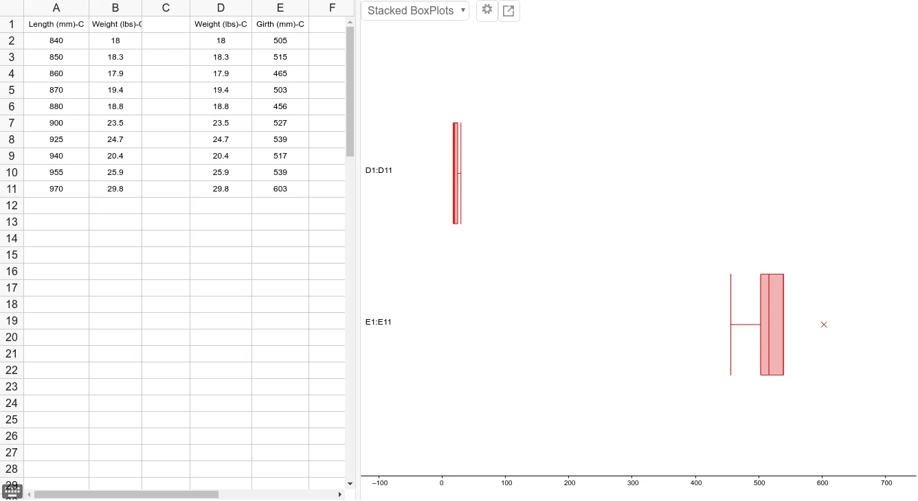
①This GeoGebra example demonstrates a comprehensive statistical analysis scene combining box plots, text annotations, sine curves, secant lines, and centroids, showing how data distribution can be visualized alongside geometric constructs. ②Core mathematical concepts include statistical characteristics (median, quartiles, mean), box plot construction, linear equations and secant line slopes, centroid/barycenter, and sine functions. ③Construction highlights: The BoxPlot command is used to generate box plots, Text command adds labels; objects A1 to B11 and D1 to E9 represent multiple points for data, auxiliary lines, and annotations, likely allowing dynamic updates via sliders or input data. ④Suitable for high school or college statistics courses, this example helps students understand data visualization, distribution shapes, and their interplay with function graphs, and serves as a teaching tool for demonstrating statistical and geometric integration.