
Linear Regression & Geometry Interactive Demo
Loading the math board and drawing, please wait…
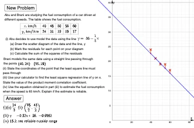
This example demonstrates the integration of linear regression models with geometric figures (like trapezoids, angles) through interactive GeoGebra constructions. It covers core math concepts including linear regression, function graphing, statistics, and residual analysis. GeoGebra commands like RandomElement, Random, Sequence, Length, ResidualPlot, PMCC, FitLineY, etc., are used in its construction, making it suitable for high school and above mathematics education and data analysis introduction.
GeoGebra Commands & Parameters
RandomElement({1 / 3, 1 / 3}) → mRandom(33, 37) → cSequence(40, 60, 5) → lxLength(lx) → nxSequence((Element[lx, i], f(Element[lx, i])), i, 1, nx) → l5Sequence(round(y(Element[l5, i]) + ((-1)^(Random[1, 2]) * Random[0, 1])), i, 1, nx) → ly1Sequence((Element[lx, i], Element[ly1, i]), i, 1, nx) → l1Random(0, 10) → aResidualPlot(l1, f) → l2Sequence(y(Element[l2, i]), i, 1, nx) → l3Sequence(Element[l3, i]^(2), i, 1, nx) → l4Sum(l4) → bSequence(Segment[Element[l1, i], Element[l5, i]], i, 1, nx) → l6PMCC(l1) → dRandomElement({30, 35, 65}) → eFitLineY(l1) → gJoin({{"x, km/h"}, lx}) → l8Join({{"y, km/litre"}, ly1}) → l9TableText(l8, l9, "c|_") → text4TableText(l7) → text9Midpoint(Element[l7, 1], Element[l7, 2]) → A
AI Drawing Prompt Reference
Create an interactive demo showing linear regression with geometric figures. Include randomly generated slope and intercept, display data points, fitted line, and residual plot. Highlight key statistics like PMCC, connect data points to form shapes, and label all elements clearly.
The prompt above was compiled from the original drawing commands and is for reference only.