Slope of a Fitted Line: A Linear Regression Practice

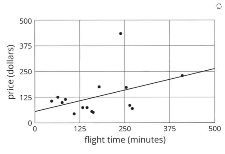
This example demonstrates how to fit a best-fit straight line to a set of data points using linear regression, and how to interpret the slope of the fitted line as a quantitative description of the overall trend. Key ideas include linear regression, the least-squares fitting principle, and the geometric meaning of a line’s slope (rate of change). Construction focuses on setting up the base objects needed for the diagram (objects A and B) and organizing the visualization in the figure (pic1), then using the fitted line generated from the data to extract and display the slope information. Suitable for upper secondary to early university learners, and useful for lessons that connect statistics with graphing and for students practicing the interpretation of regression parameters.