Visualizing Definite and Indefinite Integrals by VINOTH

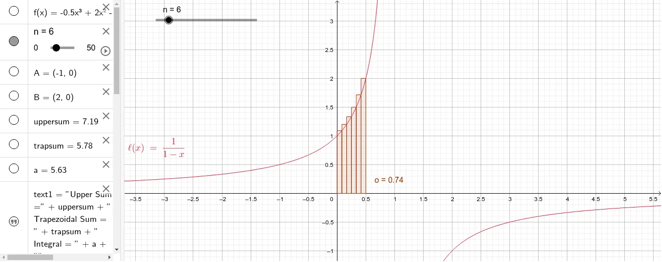
① This GeoGebra example dynamically demonstrates the geometric meaning of definite and indefinite integrals, including the area under a function curve, Riemann sum approximations, and the behavior of the integral function. ② Core mathematical concepts include definite integrals (area accumulation), indefinite integrals (antiderivatives), Riemann sums (upper rectangle and trapezoidal sums), interval partitioning, and the fundamental theorem linking integration and differentiation. ③ Construction highlights: Point defines interval endpoints, UpperSum and TrapezoidalSum generate upper rectangle and trapezoidal approximations, Integral directly plots the definite integral area, IntegralBetween computes area between two functions, Intersect finds intersection points, and a slider n controls the number of subdivisions to animate the approximation process. Objects include function f, interval points A and B, sum values, and text labels. ④ Suitable for senior high school and introductory university calculus, this example helps students intuitively grasp the definition of integrals, approximation methods, and the relationship between definite and indefinite integrals, ideal for classroom demonstrations or self-study.