
Standard Deviation Calculation: Visualizing Data Spread
Loading the math board and drawing, please wait…
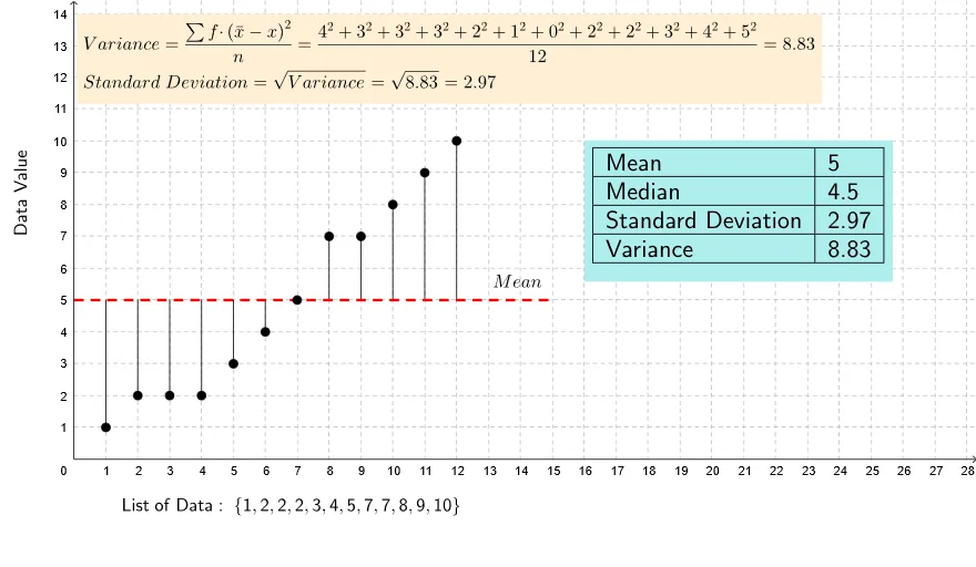
① This GeoGebra example dynamically demonstrates the calculation of standard deviation for a set of data points, visualizing the distribution and dispersion of the data. ② Core mathematical concepts include standard deviation (population standard deviation via stdevp), mean, median, and the geometric relationship between data points and the mean line. ③ Construction highlights: uses GeoGebra commands such as mean, stdevp, Point, Segment, OrthogonalLine, Intersect, TableText, and RotateText; manages data through lists list1 and list3; creates objects like points A1-A12 and B1-B13 to represent data and auxiliary elements. ④ Suitable for middle school statistics lessons to help students grasp the meaning and calculation of standard deviation, and also useful for introductory college statistics courses as a visual aid.
GeoGebra Commands & Parameters
mean(B1:B12) → B13OrthogonalLine(A, f) → gOrthogonalLine(B, f) → hOrthogonalLine(C, f) → iOrthogonalLine(D, f) → jOrthogonalLine(E, f) → kOrthogonalLine(F, f) → lOrthogonalLine(G, f) → mOrthogonalLine(H, f) → nOrthogonalLine(I, f) → pOrthogonalLine(J, f) → qOrthogonalLine(K, f) → rOrthogonalLine(L, f) → sIntersect(f, g) → MIntersect(f, h) → NIntersect(f, i) → OIntersect(f, j) → PIntersect(f, k) → QIntersect(f, l) → RIntersect(f, m) → SIntersect(f, n) → TIntersect(f, p) → UIntersect(f, q) → VIntersect(f, r) → WSegment(A, M) → tSegment(B, N) → aSegment(C, O) → bSegment(D, P) → cSegment(E, Q) → dSegment(F, R) → eSegment(S, G) → f_1Segment(T, H) → g_1Segment(I, U) → h_1Segment(V, J) → i_1Segment(W, K) → j_1Intersect(f, s) → ZSegment(L, Z) → k_1stdevp(list2) → B15Median(B1:B12) → B14Intersect(f, yAxis) → A_1Point(f) → B_1Segment(A_1, B_1) → l_1Name(Standard) → C1TableText({{A13, B13}, {A14, B14}, {A15, B15}, {A16, B16}}, "|_") → text6RotateText(text8, pi / 2) → text9