
Rotating a Cylinder
Loading the math board and drawing, please wait…
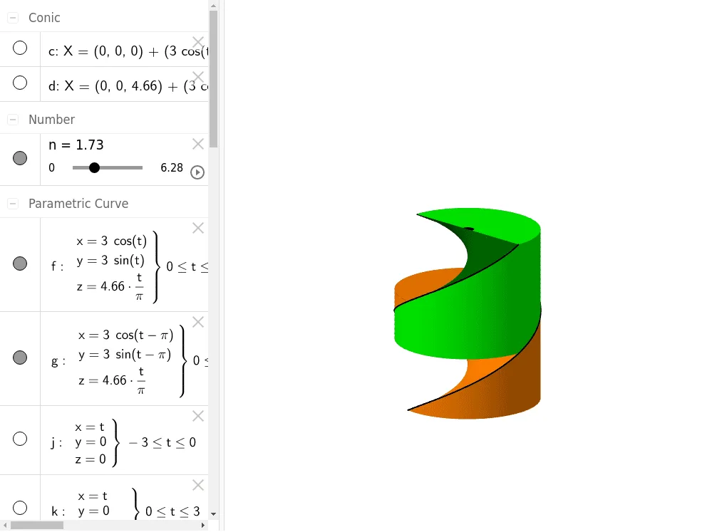
This example demonstrates the process of generating a 3D cylinder by rotating a 2D curve. Key math concepts include solids of revolution, parametric equations, and 3D geometry. Construction highlights the use of GeoGebra commands/objects like Intersect, Point, Circle, Cylinder, Surface, CurveCartesian, and Translate. Suitable for high school and above students studying applications of 3D geometry and parametric equations.
GeoGebra Commands & Parameters
Intersect(zAxis, xOyPlane) → APoint(zAxis) → BCircle(A, 3, zAxis) → cCylinder(c, z(B)) → a, d, bSurface((u * cos(t)), (u * sin(t)), (z(B) * t / π), t, 0, π, u, -3, 3) → eCurveCartesian((3 * cos(t)), (3 * sin(t)), (z(B) * t / π), t, 0, π) → fCurveCartesian((3 * cos(t - π)), (3 * sin(t - π)), (z(B) * t / π), t, 0, π) → gSurface(f, π, zAxis) → hSurface(g, π, zAxis) → iCurveCartesian(t, 0, z(B), t, 0, 3) → kSurface(k, π, zAxis) → lCurveCartesian(t, 0, 0, t, -3, 0) → jSurface(j, π, zAxis) → mTranslate(Rotate[l, n, zAxis], Vector[(0, 0, (z(B) * n / π))]) → oTranslate(Rotate[i, n, zAxis], Vector[(0, 0, (z(B) * n / π))]) → pTranslate(Rotate[m, n, zAxis], Vector[(0, 0, (z(B) * n / π))]) → qTranslate(Rotate[e, n, zAxis], Vector[(0, 0, (z(B) * n / π))]) → rTranslate(Rotate[f, n, zAxis], Vector[(0, 0, (z(B) * n / π))]) → sTranslate(Rotate[g, n, zAxis], Vector[(0, 0, (z(B) * n / π))]) → tSurface(CurveCartesian[t, 0, z(B), t, -3, 0], π, zAxis) → uSurface(CurveCartesian[t, 0, 0, t, 0, 3], π, zAxis) → v