
Riemann, Trapezoid, and Simpson's Methods for Numerical Integration
Loading the math board and drawing, please wait…
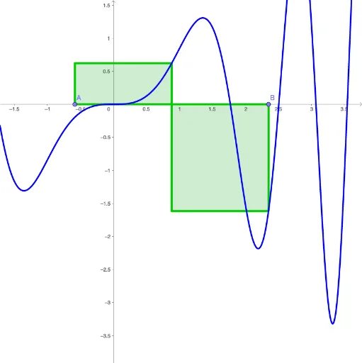
This example demonstrates numerical integration methods including Riemann, Trapezoid, and Simpson's methods. It constructs geometric figures to illustrate the core mathematical concepts. GeoGebra commands such as Point, LeftSum, TrapezoidalSum, and RectangleSum are used to create Riemann sums, trapezoidal sums, and Simpson's sums. Suitable for high school mathematics education, particularly in calculus and numerical analysis.
GeoGebra Commands & Parameters
Point(xAxis) → BPoint(xAxis) → ALeftSum(f, x(A), x(B), subintervals) → LeftRiemannLowerSum(f, x(A), x(B), subintervals) → LowerRiemannUpperSum(f, x(A), x(B), subintervals) → UpperRiemannTrapezoidalSum(f, x(A), x(B), subintervals) → TrapezoidRuleSequence((x(A) + (n * dx), 0), n, 0, subintervals) → bottomsSequence((x(Element[bottoms, n]), f(x(Element[bottoms, n]))), n, 2, subintervals + 1) → topRightSequence((x(Element[bottoms, n - 1]), f(x(Element[bottoms, n]))), n, 2, subintervals + 1) → topLeftSequence(Polygon[Element[bottoms, n], Element[bottoms, n + 1], Element[topRight, n], Element[topLeft, n]], n, 1, subintervals) → RRRectSum(Sequence[(Element[RRRect, n] * sgn(y(Element[topRight, n]))), n, 1, subintervals]) → RightRiemannSequence((x(A) + (n * dx), f(x(A) + (n * dx))), n, 0, subintervals) → topsSequence(FitPoly[{Element[tops, (2 * n) - 1], Element[tops, (2 * n)], Element[tops, (2 * n) + 1]}, 2], n, 1, subintervals / 2) → parabolasRectangleSum(f, x(A), x(B), subintervals, RiemannLeftRight) → VariableRiemannSequence(Integral[Element[parabolas, n], x(Element[tops, (2 * n) - 1]), x(Element[tops, (2 * n) + 1])], n, 1, subintervals / 2) → ShowParabolasTextfield(f) → inputBox1