
Geometric Numerical Approximation of Definite Integrals: Left/Right/Midpoint and
Loading the math board and drawing, please wait…
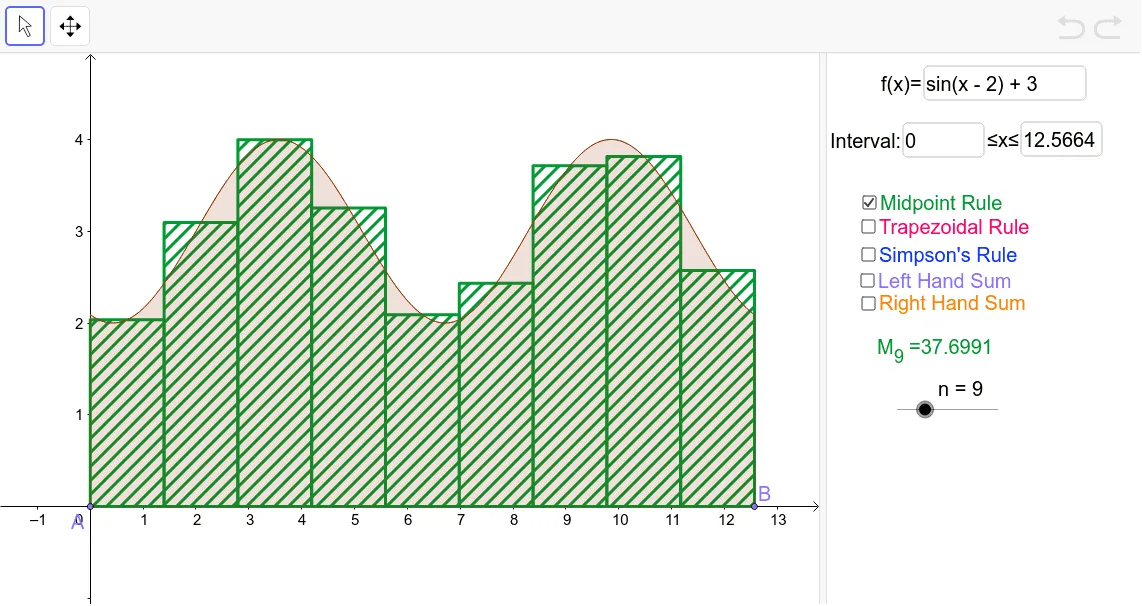
This example visually demonstrates how to approximate the area under a function curve—i.e., a definite integral—using several numerical integration schemes. It compares left- and right-endpoint Riemann sums, midpoint approximations, and the trapezoidal method by partitioning the interval [a,b] into n subintervals with step size dx and constructing the corresponding rectangles/trapezoids. Key math concepts include the geometric interpretation of the definite integral, Riemann sums, discrete summation, and numerical integration accuracy as the partition is refined. In GeoGebra, the construction relies on commands such as Function (define the integrand f/g), Sequence (generate sample points like xx and midpoints such as xmidpts), Sum (assemble the approximation), and Integral (provide the exact/target integral reference). The logic uses If and LeftSum to switch between summation variants, while graphical elements like rectangle/trapezoid point sets (e.g., mptrects, traps, pts) and lists (list1/list2/list3) manage the visualization of the approximating shapes. It is well-suited for high school and early undergraduate calculus classes, especially for teaching integral approximations and error intuition with interactive parameters.
GeoGebra Commands & Parameters
Function(f, x(A), x(B)) → gSequence(a + (k * dx), k, 0, n) → xxSequence(a + (k / 2 * dx), k, 1, (2 * n) - 1, 2) → xmidptsSequence(f(Element[xmidpts, k]), k, 1, n) → ymidptsSequence(Polygon[(Element[xx, k], 0), (Element[xx, k + 1], 0), (Element[xx, k + 1], Element[ymidpts, k]), (Element[xx, k], Element[ymidpts, k])], k, 1, n) → mptrectsSum(mptrects) → cIntegral(f, a, b) → dSequence(Polygon[(Element[xx, k], 0), (Element[xx, k + 1], 0), (Element[xx, k + 1], f(Element[xx, k + 1])), (Element[xx, k], f(Element[xx, k]))], k, 1, n) → trapsSequence((Element[xx, k], f(Element[xx, k])), k, 1, n + 1) → ptsSequence(FitPoly[{Element[pts, k], Element[pts, k + 1], Element[pts, k + 2]}, 2], k, 1, n - 1, 2) → list1Sequence(Integral[Element[list1, (k + 1) / 2], Element[xx, k], Element[xx, k + 2]], k, 1, n - 1, 2) → list2Textfield(f) → inputBox1If(h ≟ true, e = false) → jIf(h ≟ true, i = false) → kIf(h ≟ true, e = false) → lIf(h ≟ true, i = false) → mIf(h ≟ true, e = false) → oIf(h ≟ true, i = false) → pIf(h ≟ true, e = false) → qIf(h ≟ true, i = false) → rIf(h ≟ true, e = false) → sIf(h ≟ true, i = false) → tIf(h ≟ true, e = false) → uIf(h ≟ true, i = false) → vIf(h ≟ true, e = false) → wIf(h ≟ true, i = false) → zSequence(Segment[(a + (k * dx), 0), (a + (k * dx), f(a + (k * dx)))], k, 1, n, 2) → list3LeftSum(f, x(A), x(B), n) → a_1Sequence(Polygon[(Element[xx, k], 0), (Element[xx, k + 1], 0), (Element[xx, k + 1], f(Element[xx, k + 1])), (Element[xx, k], f(Element[xx, k + 1]))], k, 1, n) → rightsumTextfield(a) → inputBox2Textfield(b) → inputBox3
AI Drawing Prompt Reference
Draw the curve of function f(x) over interval [a,b] and partition it into n equal subintervals. In each subinterval, construct rectangles using left endpoints, right endpoints, midpoints, and trapezoids. All rectangles and trapezoids are placed below the curve to show approximate areas. Also display the exact integral value and compare the areas of left and right Riemann sums, midpoint approximation, and trapezoidal method. Adjusting a, b, and n allows visualization of how approximations converge to the exact value as the partition refines.
The prompt above was compiled from the original drawing commands and is for reference only.