
Definite Integral Introduction and Approximation
Loading the math board and drawing, please wait…
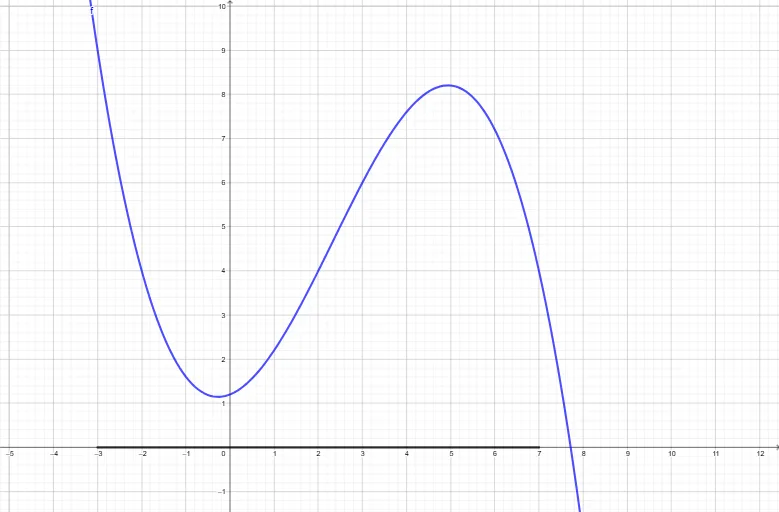
This GeoGebra example demonstrates the geometric meaning of a definite integral over a closed interval and its numerical approximation using rectangular sums. Core mathematical concepts include definite integrals, Riemann sums, function graphs, interval partitioning, and limit-based approximation. The construction employs GeoGebra commands such as Textfield, Sequence, Integral, Sum, and Segment, with InputBox objects controlling the function f, lower and upper limits a and b, and the number of rectangles n. It generates left, right, and midpoint rectangle approximations (Dx, Lr, Lh, L, etc.) and displays explanatory text labels to visualize convergence. Suitable for high school calculus introductions and undergraduate mathematical analysis courses, ideal for classroom demonstrations of integral definition and numerical approximation.
GeoGebra Commands & Parameters
Textfield(f) → InputBox1Textfield(a) → InputBox2Textfield(b) → InputBox3Textfield(n) → InputBox4Sequence(Polygon[(a + (k * Dx), 0), (a + (k * Dx), f(a + (k * Dx))), (a + ((k + 1) * Dx), f(a + (k * Dx))), (a + ((k + 1) * Dx), 0)], k, 0, n - 1) → LrSequence(f(a + (k * Dx)), k, 0, n - 1) → Lh, {9, 1.5999999999999996, 2.2, 6, 8.2}Sequence(f(a + (k * Dx)), k, 1, n) → Rh, {1.5999999999999996, 2.2, 6, 8.2, 4}Sequence(Polygon[(a + (j * Dx), 0), (a + (j * Dx), f(a + (j * Dx))), (a + ((j - 1) * Dx), f(a + (j * Dx))), (a + ((j - 1) * Dx), 0)], j, 1, n) → RrSequence(Polygon[(a + ((k - 1) * Dx), 0), (a + ((k - 1) * Dx), f(a + ((k - 0.5) * Dx))), (a + (k * Dx), f(a + ((k - 0.5) * Dx))), (a + (k * Dx), 0)], k, 1, n) → MrSequence(f(a + ((k - 0.5) * Dx)), k, 1, n) → Mh, {4, 1.2000000000000002, 4, 7.6, 7.2}Integral(f, a, b) → iSequence(Polygon[(a + ((k - 1) * Dx), 0), (a + ((k - 1) * Dx), f(a + ((k - 1) * Dx))), (a + (k * Dx), f(a + (k * Dx))), (a + (k * Dx), 0)], k, 1, n) → TtSequence(Polygon[(a + ((k - 1) * Dx), 0), (a + ((k - 1) * Dx), (f(a + ((k - 1) * Dx)) + f(a + (k * Dx))) / 2), (a + (k * Dx), (f(a + ((k - 1) * Dx)) + f(a + (k * Dx))) / 2), (a + (k * Dx), 0)], k, 1, n) → TrSequence(Polygon[(a + ((k - 1) * Dx), 0), (a + ((k - 1) * Dx), (f'(a + ((k - 1 / 2) * Dx)) * ((-Dx)) / 2) + f(a + ((k - 1 / 2) * Dx))), (a + (k * Dx), (f'(a + ((k - 1 / 2) * Dx)) * Dx / 2) + f(a + ((k - 1 / 2) * Dx))), (a + (k * Dx), 0)], k, 1, n) → MtSequence(Polygon[(a + ((k - 1) * Dx), 0), (a + ((k - 1) * Dx), (1 / Dx * Integral[f, a + ((k - 1) * Dx), a + (k * Dx)])), (a + (k * Dx), (1 / Dx * Integral[f, a + ((k - 1) * Dx), a + (k * Dx)])), (a + (k * Dx), 0)], k, 1, n) → AvSum(Av) → jSequence(If[a + ((k - 1) * Dx) < x < a + (k * Dx), Polynomial[{(a + ((k - 1) * Dx), f(a + ((k - 1) * Dx))), (a + ((k - 0.5) * Dx), f(a + ((k - 0.5) * Dx))), (a + (k * Dx), f(a + (k * Dx)))}]], k, 1, n) → StSequence(Segment[(a + (k * Dx), 0), (a + (k * Dx), f(a + (k * Dx)))], k, 0, n) → SsSegment((a, 0), (b, 0)) → m
AI Drawing Prompt Reference
Create a function graph illustrating the geometric interpretation of a definite integral and its numerical approximation. The graph should feature a function curve, the x-axis interval from a to b, and rectangular sums partitioning the interval into n subintervals. Specifically, include left, right, and midpoint Riemann sums, along with trapezoidal and average approximations, while displaying the actual integral area. Add explanatory text labels to visualize convergence. The construction sequence begins with setting the function and parameters, followed by plotting the curve, then generating rectangles and segments, and finally annotating the integral and labels.
The prompt above was compiled from the original drawing commands and is for reference only.