
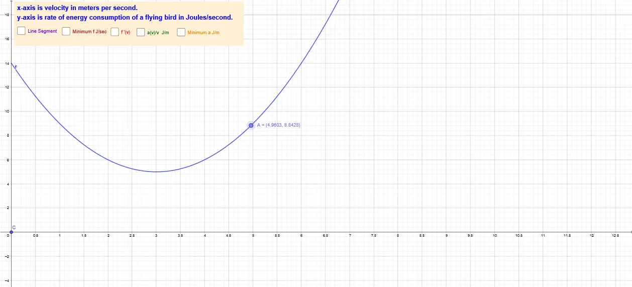
Minimizing Bird Flight Energy Consumption
Loading the math board and drawing, please wait…
This example demonstrates the mathematical optimization of bird flight energy consumption, analyzing flight paths and energy relationships. Key math concepts include calculus-based optimization, derivative applications, trigonometric functions, and linear programming. GeoGebra commands used are Point, Min, Segment, Intersect, Ray, and objects like f, A, B, g, etc. Suitable for high school students and educators focusing on mathematical modeling and physics applications.
GeoGebra Commands & Parameters
Point(f) → AMin(f(x), 0, 15) → BSegment(A, C) → gIntersect(f', h, (5.742336350493404, 2.2785337021324192)) → DIntersect(f', h, (4.933626021611028, 1.718532386013624)) → EIntersect(h, f', (5.93203383504606, 5.798541974879132)) → FIntersect(h, f', (3.741657386773968, 1.4833147735478827)) → GSegment(H, G) → iRay(C, A) → jSegment(A, I) → kSegment(B, K) → nPoint(i) → LSegment(L, C) → p
AI Drawing Prompt Reference
Draw a function curve representing bird flight energy consumption. Locate the minimum point of this function within the x-range from 0 to 15. From this minimum point, draw a segment to a moving point on the curve. From that moving point, draw a ray to a fixed point. Also plot the derivative curve of the function)Skip the derivative curve with a horizontal line, marking their intersection points. Connect two of these intersection points with a segment, and place a moving point on this segment. From this moving point, draw a segment to the fixed point. The whole figure shows the energy function, its derivative, key intersection points, and connecting segments, illustrating the optimization process.
The prompt above was compiled from the original drawing commands and is for reference only.