
Polynomials and Volumes
Loading the math board and drawing, please wait…
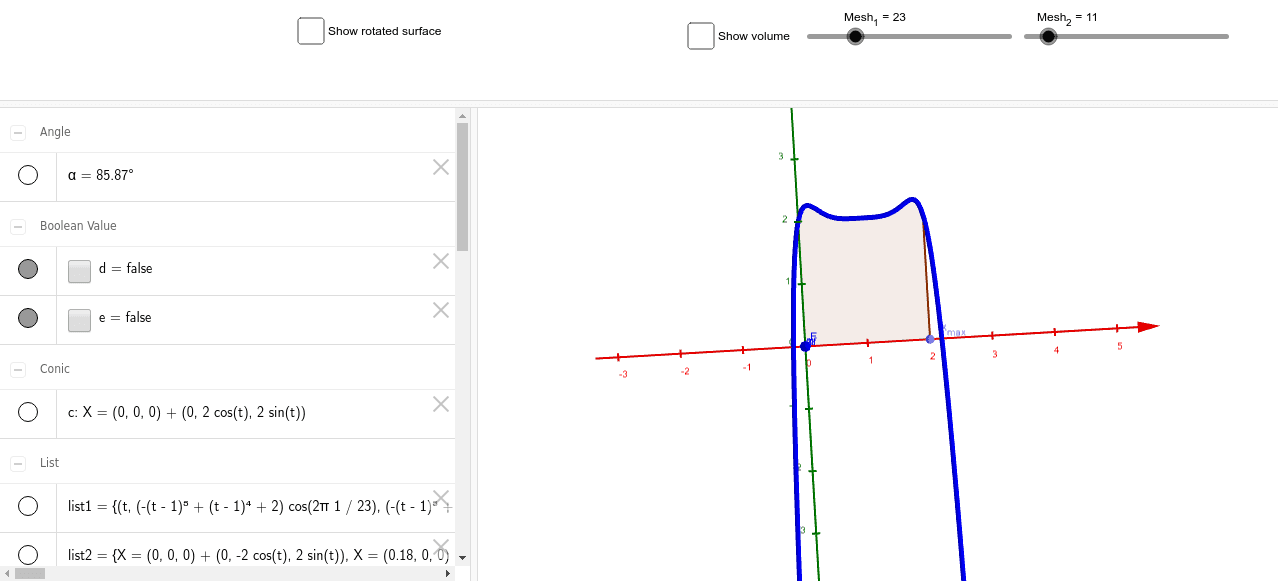
This example demonstrates the relationship between polynomial functions and volumes. Key mathematical concepts include polynomial functions and solid geometry. Using GeoGebra commands such as Intersect, Point, Line, etc., the graph of the polynomial function is constructed, and related volumes are calculated. Suitable for high school mathematics education and learning.
GeoGebra Commands & Parameters
Intersect(yAxis, zAxis) → APoint(xAxis) → BLine(A, B) → aCircle(a, C) → cPoint(c) → DPoint(a) → EAngle(C, A, D) → αCurveCartesian(t, (f(t) * cos(α)), (f(t) * sin(α)), t, 0, x(E)) → bSequence(Circle[((q * x(E) / Mesh_2), 0, 0), f((q * x(E) / Mesh_2)), x + (0 * z) = 0], q, 0, Mesh_2) → list2Sequence(CurveCartesian[t, (f(t) * cos(((2 * π) * q / Mesh_1))), (f(t) * sin(((2 * π) * q / Mesh_1))), t, 0, x(E)], q, 1, Mesh_1) → list1Append((x(E), 0), Append[(0, 0), Sequence[((x(E) * q / n_{points}), f((x(E) * q / n_{points}))), q, 0, n_{points}]]) → liste1Polygon(liste1) → poly1Rotate(poly1, α, a) → poly1'
AI Drawing Prompt Reference
Draw the graph of a polynomial function and demonstrate its relationship with volumes. Start by plotting the coordinate axes, then determine a line and a circle. Use these elements to calculate an angle. Next, draw a curve based on the angle and the polynomial function. Finally, generate multiple polygons through rotation and sequencing to illustrate the volume calculation process.
The prompt above was compiled from the original drawing commands and is for reference only.