
Polar Curves
Loading the math board and drawing, please wait…
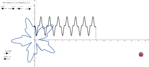
This example demonstrates the method of drawing polar curves. Key mathematical concepts include polar coordinates, parametric equations, and curve sketching. Using GeoGebra commands such as Textfield, Segment, Line, and Intersect, the generation process of polar curves can be dynamically displayed. Suitable for high school mathematics education and learning.
GeoGebra Commands & Parameters
Textfield(f) → inputBox1Segment((0, 0), D) → gLine(CC, yAxis) → hIntersect(xAxis, h) → ASegment(CC, A) → iCurveCartesian(t, f(tm - t), t, 0, tm) → c_1CurveCartesian((f(tm - t) * sin(t)), (f(tm - t) * cos(t)), t, 0, tm) → d_1
AI Drawing Prompt Reference
Draw an example of a polar curve to demonstrate how to plot using parametric equations. Start by drawing a segment from the origin to a point on a horizontal line, then find their intersection and connect the origin to this point. Next, plot two curves using parametric equations representing the sine and cosine transformations of the function values, showing the curve shape in polar coordinates.
The prompt above was compiled from the original drawing commands and is for reference only.