
Perspective View in a Sphere
Loading the math board and drawing, please wait…
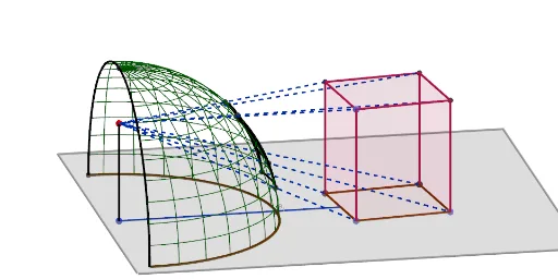
This example demonstrates a perspective view within a sphere. Key mathematical concepts include geometric transformations and rotation. Using GeoGebra commands such as Line, Circle, Segment, and Point, the perspective view within a sphere is constructed. Suitable for high school mathematics education, particularly in solid geometry and geometric transformations.
GeoGebra Commands & Parameters
Line(A, zAxis) → fCircle(A, R, f) → cSegment(B, A) → gPoint(g) → CCircumcircleArc(T, B_1, U) → e_2Polygon(I, K, L, F) → q1, i_3, k_3, l_3, f_3Sphere(A, R) → ePointIn(q1) → DPointIn(q1) → EPolygon(D, E, 4, q1) → poly1, i, j, k, l, G, HLine(E, f) → mPoint(m) → JPrism(poly1, (-Distance[J, E])) → a, M, arêteDM, arêteEN, arêteGO, arêteHP, arêteMN, arêteNO, arêteOP, arêteMP, N, O, P, faceDENM, faceEGON, faceGHPO, faceDHPM, faceMNOPMidpoint(P, M) → QMidpoint(H, D) → SMidpoint(H, P) → VMidpoint(M, D) → WRay(P, C) → nRay(Q, C) → pRay(M, C) → qRay(V, C) → rRay(H, C) → sRay(D, C) → tRay(S, C) → bRay(W, C) → dRay(M, C) → f_1Intersect(n, e) → Z, A_1Intersect(p, e) → C_1, D_1Intersect(f_1, e) → E_1, F_1Intersect(r, e) → G_1, H_1Intersect(d, e) → I_1, J_1Intersect(s, e) → K_1, L_1Intersect(b, e) → M_1, N_1Intersect(t, e) → O_1, P_1CircumcircleArc(Z, C_1, E_1) → c_1CircumcircleArc(E_1, I_1, O_1) → d_1CircumcircleArc(Z, G_1, K_1) → e_1CircumcircleArc(O_1, M_1, K_1) → g_1Midpoint(J, O) → Q_1Midpoint(O, G) → R_1Midpoint(J, E) → S_1Ray(J, C) → h_1Ray(O, C) → i_1Ray(Q_1, C) → j_1Ray(G, C) → k_1Ray(E, C) → l_1Midpoint(E, G) → T_1Ray(R_1, C) → m_1Ray(S_1, C) → n_1Intersect(h_1, e) → U_1, V_1Intersect(j_1, e) → W_1, Z_1Intersect(n_1, e) → A_2, B_2Intersect(i_1, e) → C_2, D_2Intersect(l_1, e) → E_2, F_2Intersect(m_1, e) → G_2, H_2Intersect(k_1, e) → I_2, J_2Ray(T_1, C) → p_1Intersect(p_1, e) → K_2, L_2CircumcircleArc(C_2, W_1, U_1) → q_1CircumcircleArc(U_1, A_2, E_2) → r_1CircumcircleArc(C_2, G_2, I_2) → s_1CircumcircleArc(E_2, K_2, I_2) → t_1Midpoint(arêteOP) → M_2Midpoint(arêteMN) → N_2Midpoint(k) → O_2Midpoint(i) → P_2Ray(O_2, C) → a_1Ray(P_2, C) → b_1Ray(N_2, C) → f_2Ray(M_2, C) → g_2Intersect(f_2, e) → Q_2, R_2Intersect(g_2, e) → S_2, T_2Intersect(b_1, e) → U_2, V_2Intersect(a_1, e) → W_2, Z_2CircumcircleArc(U_1, Q_2, E_1) → c_2CircumcircleArc(O_1, U_2, E_2) → d_2CircumcircleArc(Z, S_2, C_2) → h_2CircumcircleArc(K_1, W_2, I_2) → k_2Segment(A, T_1) → i_2Segment(C, P) → j_2Segment(C, O) → l_2Segment(C, M) → m_2Segment(C, J) → n_2Segment(C, H) → p_2Segment(C, D) → q_2Segment(C, E) → s_2Segment(C, G) → r_2Segment(C, A) → t_2Sequence(CurveCartesian[x(A) + ((R * cos(k)) * cos(j)), y(A) + ((R * cos(k)) * sin(j)), z(A) + (R * sin(k)), j, ((-π)) / 2, π / 2], k, 0, π / 2, π / oo) → l2CircumcircleArc(T, B, U) → c_3Sequence(CurveCartesian[x(A) + ((R * cos(k)) * cos(j)), y(A) + ((R * cos(k)) * sin(j)), z(A) + (R * sin(k)), k, 0, π / 2], j, ((-π)) / 2, π / 2, (2 * π / (oo + 10))) → l1CircumcircleArc(U_1, Q_2, E_1) → d_3CircumcircleArc(O_1, U_2, E_2) → e_3CircumcircleArc(C_2, S_2, Z) → h_3CircumcircleArc(K_1, W_2, I_2) → g_3