
Pedagogical Pendulum: Dynamic Time-Angle Simulation
Loading the math board and drawing, please wait…
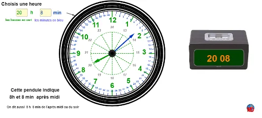
This GeoGebra example constructs a pedagogical pendulum model that dynamically simulates the relationship between the pendulum's swing, clock hand positions, time, and angles. Core mathematical concepts include angle measurement, trigonometric functions (cosine), vector rotation, sequences and series, linear equations, and modular arithmetic. The construction uses commands such as Textfield for input, Sequence for generating lists, Rotate and Vector for rotational and vector operations, Circle for the clock face, Mod for modular arithmetic, If for conditional logic, and Point for defining key points. Key objects include r (radius), A (center), m1/h1 (minute/hour hands), th1 (angle), B, tm1, multiple lists (liste1-8), and various text and image elements. This resource is suitable for middle or high school mathematics and physics classes to teach angles, periodic motion, and function graphs, as well as for exploring clock reading and angle conversion.
GeoGebra Commands & Parameters
Textfield(h1) → th1Textfield(m1) → tm1Sequence(Rotate[B, (-i), A], i, 0, 6.28319, 0.10472) → liste1Sequence(Rotate[B - (0, 0.125), (-i), A], i, 0, 6.28319, 0.10472) → liste2Sequence(Segment[Element[liste1, i], Element[liste2, i]], i, 1, Length[liste1]) → liste3Sequence(Rotate[B, (-i), A], i, 0, 6.283185307179586, 0.5235987755982988) → liste4Sequence(Rotate[B - (0, 0.3), (-i), A], i, 0, 6.28319, 0.5236) → liste5Sequence(Segment[Element[liste4, i], Element[liste5, i]], i, 1, Length[liste5]) → liste6Rotate(B - (0, 1.1), (((-h1) * 2) * π / 12) - ((m1 * 2) * π / 840), A) → CVector(A, C) → uRotate(B - (0, 0.65), (((-m1) * 2) * π / 60), A) → DVector(A, D) → wSequence(Rotate[B - (0.185, 0.6), (-i), A - (0.145, 0.095)], i, 0, 6.28319, 0.5236) → liste8Sequence(Text[i, Element[liste8, i + 1]], i, 1, Length[liste8] - 1) → liste7Circle(A, r) → cCircle(A, r + 0.081) → dCircle(A, r + 0.182) → eCircle(A, r + 0.25) → fCircle(A, r + 0.325) → gCircle(A, r + 0.35) → hCircle(A, r + 0.395) → kMod(a, 2) → aaIf(h1 > 12, h1 - 12, h1) → hhCircle(A, r + 0.515) → pCircle(A, r / 12) → qSequence(Rotate[B - (0.1, 0.9), (-i), A - (0.102, 0.02)], i, 0, 6.28319, 0.5236) → l2Sequence(Text[12 + i, Element[l2, i + 1]], i, 1, Length[liste8] - 1) → l1Sequence(Rotate[B - (-0.142, 0.262), (-i), A + (-0.072, -0.02)], i, 0, 6.28319, 0.10472) → liste2bSequence(Text[i, Element[liste2b, i]], i, 1, Length[liste2b] - 1) → l3Circle(A, C) → sSequence(Rotate[L, (-i), A], i, 0, 6.28319, 0.5236) → l4Sequence(Rotate[L - (0, 0.3), (-i), A], i, 0, 6.28319, 0.5236) → l5Sequence(Segment[Element[l4, i], A], i, 1, Length[l4]) → l6Point(p) → NVector(M, N) → v
AI Drawing Prompt Reference
Create a dynamic simulation showing the relationship between a pendulum's swing and clock hand positions over time. Include a circular clock face with two hands, a shorter minute hand and a longer hour hand. Visualize the pendulum's swing path and use concentric circles to represent different time units. Add number markings and angle measurements to illustrate the connection between pendulum swing angles and time, as well as how hand positions change over time, emphasizing periodic motion and angle calculations.
The prompt above was compiled from the original drawing commands and is for reference only.