
P-Value and Critical Value Comparison
Loading the math board and drawing, please wait…
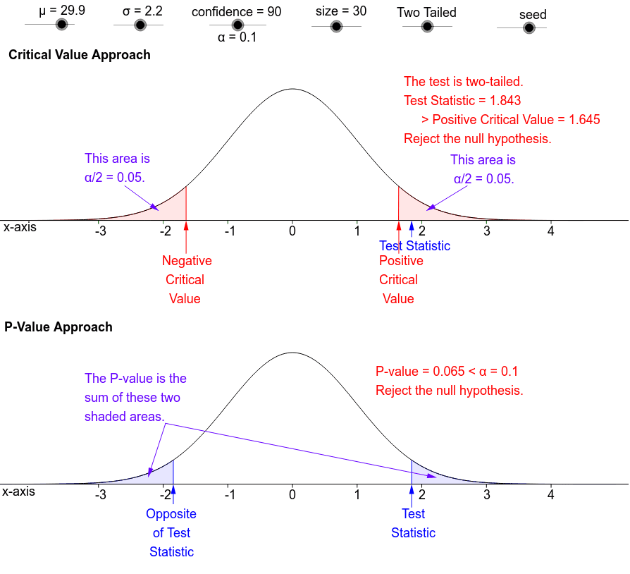
This example demonstrates the comparison between the critical value approach and the P-value approach in hypothesis testing. It involves core concepts like hypothesis testing, P-values, critical values, and normal distributions. The construction utilizes GeoGebra commands and objects such as Sequence, Append, Element, Mean, Integral, Line, Vector, If, IntegralBetween, and Text to visualize normal curves, sample means, critical values, and P-values. It is suitable for high school and above students learning about statistical methods.
GeoGebra Commands & Parameters
Sequence(k, k, 80, 99) → CL1Append(CL1, 99.9) → CL2Element(CL2, cs) → ConfidenceSequence(RandomNormal[μ + Type - 2 + seed, σ], k, 1, size) → SampleMean(Sample) → xbarIntegral(BellCurve, TstSt, 10) → PVhiIntegral(BellCurve, -10, TstSt) → PVloLine((-5, 0), (5, 0)) → XAx2Vector(TST2, TSH2) → TSV1If(Type ≟ 2, (-InverseNormal[0, 1, α / 2]), (-InverseNormal[0, 1, α])) → CVhiVector(TST1, TSH1) → TSV2If(Type ≟ 2, InverseNormal[0, 1, α / 2], InverseNormal[0, 1, α]) → CVloVector(CVT2, CVH2) → CVVhiIntegral(exp((-x^(2))) / ((4 * 3.141592653589793)), TstSt, 10) → MhixIntegral((x * e^(((-x^(2))) / 2) / sqrt((2 * 3.141592653589793))), TstSt, 10) → MhiyVector(CVT1, CVH1) → CVVloIntegral(exp((-x^(2))) / ((4 * 3.141592653589793)), -10, TstSt) → MloxIntegral((x * e^(((-x^(2))) / 2) / sqrt((2 * 3.141592653589793))), -10, TstSt) → MloyVector(A, CMlo) → PVVloVector(B, CMhi) → PVVhiElement(TypTx, Type) → typeIntegral(exp((-x^(2))) / ((4 * 3.141592653589793)), CVhi, 10) → Mhix2Integral((x * e^(((-x^(2))) / 2) / sqrt((2 * 3.141592653589793))), CVhi, 10) → Mhiy2Vector(C, CMhi2) → AlphaRVIntegral(exp((-x^(2))) / ((4 * 3.141592653589793)), -10, CVlo) → Mlox2Integral((x * e^(((-x^(2))) / 2) / sqrt((2 * 3.141592653589793))), -10, CVlo) → Mloy2Vector(D, CMlo2) → AlphaRCMIntegral(BellCurve, -5, (-abs(TstSt))) → TTLfIntegral(BellCurve, abs(TstSt), 5) → TTRtIntegral(exp((-x^(2))) / ((4 * 3.141592653589793)), -10, (-abs(TstSt))) → Mlox3Integral((x * e^(((-x^(2))) / 2) / sqrt((2 * 3.141592653589793))), -10, (-abs(TstSt))) → Mloy3Integral(BellCurve, -10, (-abs(TstSt))) → MTTLIntegral(exp((-x^(2))) / ((4 * 3.141592653589793)), abs(TstSt), 10) → Mhix3Integral((x * e^(((-x^(2))) / 2) / sqrt((2 * 3.141592653589793))), abs(TstSt), 10) → Mhiy3Vector(E, CMlo3) → TTLVVector(E, CMhi3) → vVector(F, CMlo4) → AHLVVector(G, CMhi4) → AHHVVector(OTSLP, OTSP) → uSequence(Segment[(k, (-0.01)), (k, 0)], k, -3, 4) → XTcSq2Sequence(Text[k, (k - 0.05, (-0.045))], k, -3, 4) → XLbTxSq2Line((-5, 0.8), (5, 0.8)) → XAx1Sequence(Segment[(k, 0.79), (k, 0.8)], k, -3, 4) → XTcSq1Sequence(Text[k, (k - 0.05, 0.755)], k, -3, 4) → XLbTxSq1IntegralBetween(BellCurve2, 0.8, CVhi, 4.5) → AlFlRtIntegralBetween(BellCurve2, 0.8, -5, CVlo) → AlFlLfIntegralBetween(BellCurve2, 0.8, -5, CVlo) → AlHfLfIntegralBetween(BellCurve2, 0.8, CVhi, 4.5) → AlHfRtText("Test Statistic", (TstSt - 0.5, 0.71)) → TSLab2