
Octonion Multiplication Chart and Fano Plane
Loading the math board and drawing, please wait…
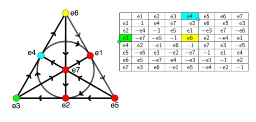
This example demonstrates the geometric representation of octonion multiplication charts and the Fano plane. Key mathematical concepts include octonion multiplication rules, the geometric structure of the Fano plane, and polygon construction. GeoGebra commands used in the construction are: Polygon, Incircle, Center, Intersect, Segment, CircumcircleArc, CircleArc, Point, Tangent, UnitVector, Dilate, TableText, Sequence, IndexOf, Element. It is suitable for high school students and above, mathematics enthusiasts, and researchers studying the relationship between octonions and the Fano plane for educational demonstrations or mathematical exploration.
GeoGebra Commands & Parameters
Polygon(e3, e5, 3) → poly1, f, g, h, e6Incircle(e3, e5, e6) → cCenter(c) → e7Intersect(c, f) → e2, HIntersect(c, g) → e1,Intersect(c, h) → e4,Segment(e5, e7) → iSegment(e7, e4) → jSegment(e6, e7) → kSegment(e7, e2) → lSegment(e3, e7) → mSegment(e7, e1) → nSegment(e4, e6) → pCircumcircleArc(e6, A, e3) → dCircleArc(e7, e1, e4) → eCircleArc(e7, e4, e2) → qCircleArc(e7, e2, e1) → rSegment(e6, e1) → sSegment(e1, e5) → tSegment(e5, e2) → aSegment(e2, e3) → bPoint(e) → BPoint(r) → CPoint(q) → DTangent(D, q) → f_1,UnitVector(f_1) → uSegment(D, D + (0.1 * u)) → g_1Tangent(B, e) → h_1,UnitVector(h_1) → vSegment(B, B + (0.1 * v)) → i_1Tangent(C, r) → j_1,UnitVector(j_1) → wSegment(C, C + (0.1 * w)) → k_1Dilate(e5, 0.6, e7) → e5'Dilate(e7, 0.6, e7) → e7'Segment(e5', e7') → i'Dilate(e6, 0.6, e7) → e6'Dilate(e7, 0.6, e7) → e7'_1Segment(e6', e7'_1) → k'Dilate(e3, 0.6, e7) → e3'Dilate(e7, 0.6, e7) → e7'_2Segment(e3', e7'_2) → m'Tangent(A, d) → l_1,UnitVector(l_1) → u_1Segment(A, A - (0.1 * u_1)) → m_1Segment(e3, e4) → n_1TableText({R0, R1, R2, R3, R4, R5, R6, R7}, "c_|h") → text1Sequence(G + (w * (F - G)), w, 0, 1, 1 / 6) → L_1Point(L_1) → ISequence(M + (w * (N - M)), w, 0, 1, 1 / 6) → L_2Point(L_2) → OPolygon((x(O), y(I)), (x(O), y(K)), (x(R), y(K)), (x(R), y(I))) → q1, r_1, s_1, t_1, a_1Polygon({I, J, K, L}) → p_1Polygon({O, P, Q, R}) → q_1IndexOf(O, L_2) → oIndexOf(I, L_1) → b_1Element(Element[L3, b_1], o) → text2
AI Drawing Prompt Reference
Draw a geometric representation of an octonion multiplication chart and the Fano plane, including a triangle and its incircle, along with multiple intersection points and line segments. Start by drawing the triangle and its incircle, then determine the center and connect it to the vertices of the triangle. Next, mark the intersection points on the circle and draw line segments connecting these points. Finally, add arcs and tangents to create a complex geometric structure, showcasing the relationship between octonion multiplication rules and the Fano plane.
The prompt above was compiled from the original drawing commands and is for reference only.