Numerical Integration for Free Fall

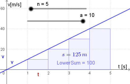
This example demonstrates free-fall motion under constant gravitational acceleration by visualizing how velocity and displacement evolve over time. It emphasizes the accumulation idea behind integration: displacement is obtained as the integral (numerically approximated by sums) of velocity over time. The key math concepts include discretization with a time step, piecewise summation, and the Riemann-sum viewpoint using LowerSum to approximate an integral. Construction uses GeoGebra commands LowerSum and Sequence to generate the time partition and sample values; objects such as a, v, and s represent acceleration, velocity, and displacement (or their corresponding functions/series). Variables like n and l1 support the interval sizing, while B2–B10 and B1 store boundary/segment-related values and A1–A10 hold computed sub-interval points/results. Text labels (text1) help explain the current approximation. Suitable for late high school through early university calculus and modeling lessons, especially for introducing numerical integration and connecting calculus to physical motion.