
Newton's Method for Approximating Roots of an Equation
Loading the math board and drawing, please wait…
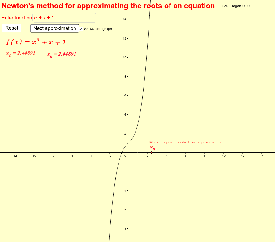
This example demonstrates how Newton's method can be used to approximate the roots of an equation. Key mathematical concepts include functions, derivatives, and iteration. Using GeoGebra commands such as Point, Derivative, and IterationList, the iterative process is dynamically illustrated. Suitable for high school mathematics education.
GeoGebra Commands & Parameters
Point(xAxis) → ADerivative(g) → g'IterationList(h, x_0, 15) → List1Element(List1, 0) → bSequence(Vector[(Element[List1, i], 0), (Element[List1, i], g(Element[List1, i]))], i, 1, m1) → List3Sequence(Vector[(Element[List1, i], g(Element[List1, i])), (Element[List1, i + 1], 0)], i, 1, n) → List4Sequence(g(Element[List1, i]), i, 1, 15) → List2Line(B, C) → dOrthogonalLine(D, xAxis) → eTextfield(g) → inputBox1
AI Drawing Prompt Reference
Draw a graph illustrating Newton's method for approximating roots. Include a function curve, an initial point, a sequence of points representing iterations, and a line connecting the initial point to the final point. The iteration process is shown through the point sequence and line, demonstrating the approach to the root from the initial value.
The prompt above was compiled from the original drawing commands and is for reference only.