
Visualizing Partial Derivatives
Loading the math board and drawing, please wait…
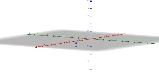
This example dynamically illustrates the concept of partial derivatives. It involves the calculation of partial derivatives of a function and how to visually understand the meaning of partial derivatives. The construction uses commands such as PointIn, Derivative, IntersectPath, Line, and Vector, suitable for university-level calculus courses.
GeoGebra Commands & Parameters
PointIn(z = 0) → ADerivative(f, x) → FxDerivative(f, y) → FyIntersectPath(p, f) → eq1IntersectPath(q, f) → eq2Line(B, Vector[(1, 0, Fx(x(A), y(A)))]) → gLine(B, Vector[(0, 1, Fy(x(A), y(A)))]) → hVector(B, B + (1, 0, Fx(x(A), y(A)))) → aVector(B, B + (0, 1, Fy(x(A), y(A)))) → b
AI Drawing Prompt Reference
Draw a graph illustrating partial derivatives. Include a function curve, a point, and two lines emanating from the point, representing partial derivatives with respect to x and y. The lines should indicate the direction of the derivatives. The graph should clearly show the concept of partial derivatives to help understand the rate of change of a function at a specific point.
The prompt above was compiled from the original drawing commands and is for reference only.