
Net of a Cone: Building the Cone’s Unfolding
Loading the math board and drawing, please wait…
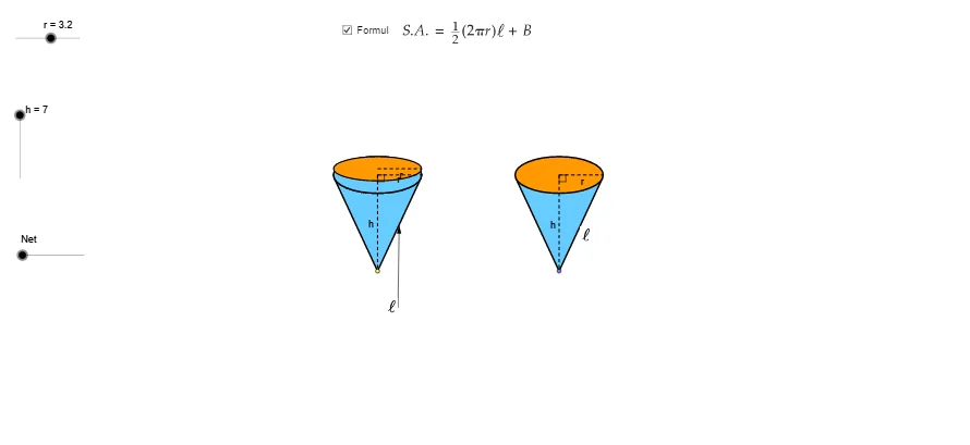
This example demonstrates how the surface of a cone can be unfolded into a planar net, emphasizing the correspondence between the cone’s lateral surface and a circular sector. The key mathematics includes the cone’s slant height (used as the sector radius), the relationship between the cone’s base circumference and the sector arc length, and the construction of the sector’s central angle from those measurements. From the construction summary, the model relies on GeoGebra commands such as Point, Line, Angle, Arc, Circle/CircleSector to generate the required arcs and boundaries, Intersect to locate key intersection points, Segment and Midpoint for defining lengths and reference points, and transformation tools like Translate, Rotate, Mirror and Vector to position and relate components of the net. Additional geometric tools including Tangent and OrthogonalLine support constraint-based layout, while Conic/Conic-related objects and Ellipse appear as intermediate geometry in the construction pipeline. Suitable for middle/high school solid geometry, 3D-to-2D unfolding visualization, and instructional demonstrations or student construction practice.
GeoGebra Commands & Parameters
Point(xAxis) → ACircle(A, r) → cIntersect(c, xAxis) → B, CEllipse(E, D, C) → eIntersect(xAxis, yAxis) → FVector(F, G) → uTranslate(B, Vector[(u * h)]) → B'_1Translate(C, Vector[(u * h)]) → C'_1Translate(A, Vector[(u * h)]) → A'_1Translate(e, Vector[(u * h)]) → e'_1Arc(e'_1, C'_1, B'_1) → p_5Arc(e'_1, B'_1, C'_1) → qSegment(A'_1, A) → h_6Segment(A'_1, C'_1) → pAngle(A, A'_1, C'_1) → αLine(A, A'_1) → jIntersect(e'_1, j) → H, ICircle(I, r) → tIntersect(t, j, 2) → KCircle(K, I) → d_1Intersect(d_1, j, 2) → NVector(H, N) → vTranslate(H, Vector[(v * n)]) → H'_1Translate(D, Vector[(u * h)]) → D'Translate(E, Vector[(u * h)]) → E'Line(B, B'_1) → lLine(C, C'_1) → mIntersect(d_1, l, 1) → PIntersect(d_1, m, 1) → QVector(B'_1, P) → zVector(C'_1, Q) → u_1Translate(B'_1, Vector[(z * n)]) → B''Translate(C'_1, Vector[(u_1 * n)]) → C''Midpoint(B'_1, A'_1) → RMidpoint(B, A) → SLine(R, S) → a_1Intersect(q, a_1) → T,Intersect(d_1, a_1, 1) → UVector(T, U) → v_1Translate(T, Vector[(v_1 * n)]) → T'If(n ≟ 0.01, B'_1, If[n < 1, B'', P]) → B_1If(n ≟ 0.01, T, If[n < 1, T', U]) → D_1If(n ≟ 0.01, H, If[n < 1, H'_1, N]) → E_1If(n ≟ 0.01, C'_1, If[n < 1, C'', Q]) → F_1Conic(B_1, D_1, E_1, F_1, I) → g_1Conic(I, B_1, D_1, E_1, F_1) → h_1OrthogonalLine(I, j) → l_1OrthogonalLine(H, j) → b_2Intersect(m, l_1) → H_2Midpoint(H_2, C'_1) → I_2OrthogonalLine(C'_1, m) → i_2Segment(K, F_1) → m_4Translate(e, Vector[(u * h)]) → e'Tangent(A, e'_1) → a, bIntersect(e', b) → J, G_2Intersect(e', a) → L, R_2Segment(A, J) → fSegment(A, L) → gCircle(I, sqrt(h^(2) + r^(2))) → kIntersect(k, j, 1) → MCircle(M, sqrt(h^(2) + r^(2))) → sSegment(M, I) → iRotate(I, γ, M) → I'_1Rotate(I, (-γ), M) → I'_2OrthogonalLine(I'_2, i_2) → b_1Intersect(b_2, b_1) → OMidpoint(H, O) → VCircle(V, O) → c_1Vector(O, I'_2) → wCenter(g_1) → WSegment(W, F_1) → e_1Vector(H, A) → w_1Translate(H, Vector[(w_1 * (n - 1))]) → H'If(n < 1, H, If[n < 2, H', A]) → ZSegment(H, Z) → f_1Rotate(I, (-δ), M) → I'Vector(L, I') → z_1Translate(c_1, Vector[(w * (n - 2))]) → k_1Center(k_1) → A_1Intersect(k_1, j) → C_1, Q_1Rotate(C_1, (180° * (n - 2)), A_1) → G_1If(n < 2, H, If[n ≤ 3, G_1, I'_2]) → H_1Mirror(H_1, j) → I_1Translate(L, Vector[(z_1 * (n - 2))]) → L'If(n < 2, L, If[n ≤ 3, L', I']) → J_1Mirror(J_1, j) → K_1Conic(I_1, H_1, J_1, I, K_1) → p_1Vector(A, M) → i_1Translate(A, Vector[(i_1 * (n - 2))]) → A'If(n < 2, A, If[n ≤ 3, A', M]) → L_1Tangent(L_1, p_1) → j_1, m_1Intersect(p_1, m_1, 1) → M_1Intersect(p_1, j_1, 1) → N_1Polygon(L_1, M_1, N_1) → poly1, n_1, l_2, m_2Arc(p_1, N_1, M_1) → q_1Line(L_1, b_2) → r_1Intersect(p_1, r_1, 1) → O_1Intersect(p_1, r_1, 2) → P_1Arc(p_1, P_1, O_1) → s_1Polygon(L_1, O_1, I_1) → poly2, i_3, l_3, o_1Polygon(L_1, H_1, P_1) → poly3, p_2, l_4, h_2Arc(p_1, O_1, I_1) → t_1Arc(p_1, H_1, P_1) → c_2Segment(L_1, I_1) → a_2Segment(L_1, H_1) → d_2Arc(p_1, H_1, I_1) → e_2Polygon(I_1, L_1, H_1) → poly4, h_3, i_4, l_5CircleSector(M, I'_2, I'_1) → f_2CircleSector(M, I'_2, I'_1) → g_2Arc(p_1, H_1, I_1) → k_2Segment(M_1, L_1) → j_2Segment(N_1, L_1) → n_2Polygon(I_1, L_1, H_1) → poly5, h_4, i_5, l_6Arc(p_1, H_1, I_1) → q_2Polygon(J, A, L) → poly6, l_7, j_3, a_3Point(xAxis) → R_1OrthogonalLine(R_1, xAxis) → r_2Intersect(i_2, r_2) → S_1Circle(R_1, r) → s_2Intersect(s_2, xAxis) → T_1, U_1OrthogonalLine(T_1, i_2) → t_2OrthogonalLine(V_1, i_2) → b_3OrthogonalLine(W_1, i_2) → c_3Intersect(i_2, t_2) → Z_1Intersect(i_2, b_3) → A_2Intersect(i_2, c_3) → B_2Ellipse(A_2, B_2, Z_1) → d_3Tangent(R_1, d_3) → e_3, f_3Intersect(d_3, f_3, 1) → C_2Intersect(d_3, e_3, 1) → D_2Polygon(C_2, D_2, R_1) → poly7, r_3, c_4, d_4Ellipse(A_2, B_2, Z_1) → g_3OrthogonalLine(U_1, xAxis) → k_3Intersect(g_3, k_3) → E_2, J_2Segment(S_1, E_2) → m_3Segment(S_1, R_1) → n_3Intersect(d_3, m_3, 1) → F_2Midpoint(g) → K_2Midpoint(f_1) → L_2Point(j) → M_2Midpoint(I_1, A') → N_2Midpoint(A', H_1) → O_2Vector(M_2, N_2) → u_2Vector(M_2, O_2) → v_2Line(M_2, r_1) → p_3Point(p_3) → P_2Vector(P_2, K_2) → z_2Vector(P_2, L_2) → u_3Center(g_3) → Q_2Angle(F_2, Q_2, R_1) → εSegment(I_1, H_1) → q_3Intersect(k_2, q_3, 2) → S_2Point(poly7) → T_2
AI Drawing Prompt Reference
Draw an unfolded cone net, showing how the lateral surface becomes a planar sector. The figure includes a circular sector (representing the unfolded cone side), a circle (representing the cone's base), and an arc connecting them. The sector's radius corresponds to the cone's slant height, and the arc length equals the base circumference. Construct by determining the radius and arc length, calculating the central angle, drawing the sector and circle, then connecting with an arc to form the complete net. Suitable for geometry teaching and visualization.
The prompt above was compiled from the original drawing commands and is for reference only.