
Mr. Lamb’s Class Pencil Length Analysis
Loading the math board and drawing, please wait…
In collections
UCSS Secondary Math I Unit 4 Lesson 1
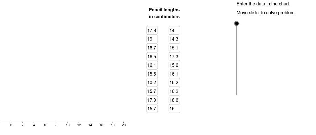
This example demonstrates how to analyze pencil length data from Mr. Lamb’s class using GeoGebra, focusing on creating dot plots, box plots, and calculating median, quartiles, and other statistical measures. Key math concepts include data sorting, statistical graphing, five-number summary, and basic probability statistics. GeoGebra commands and objects like Sort, DotPlot, Median, Q1, Q3, BoxPlot, Segment, Textfield, Element, RemoveUndefined, Circle, Conic, Join, Polygon are used for data processing and visualization. Suitable for high school mathematics teaching, particularly for introductory probability and statistics education.
GeoGebra Commands & Parameters
Sort(LambList) → SortedListDotPlot(SortedList) → DotPlotMedian(LambList) → ListMedQ1(LambList) → ListQ1Q3(LambList) → ListQ3BoxPlot(4, 1, LambList) → ListBoxSegment((ListMed, 0), (ListMed, 2.5)) → SegMedSegment((ListQ1, 0), (ListQ1, 2.5)) → SegQ1Segment((ListQ3, 0), (ListQ3, 2.5)) → SegQ3Segment((UpperLim, 0), (UpperLim, 2.5)) → SegUpperSegment((LowerLim, 0), (LowerLim, 2.5)) → SegLowerTextfield(A1) → InA1Textfield(A2) → InA2Textfield(A3) → InA3Textfield(A4) → InA4Textfield(A5) → InA5Textfield(A6) → InA6Textfield(A7) → InA7Textfield(A8) → InA8Textfield(A9) → InA9Textfield(A10) → InA10Textfield(A11) → InA11Textfield(A12) → InA12Textfield(A13) → InA13Textfield(A14) → InA14Textfield(A15) → InA15Textfield(A16) → InA16Textfield(A17) → InA17Textfield(A18) → InA18Textfield(A19) → InA19Textfield(A20) → InA20Element(SortedList, C1) → B1Element(SortedList, C2) → B2Element(SortedList, C3) → B3Element(SortedList, C4) → B4Element(SortedList, C5) → B5Element(SortedList, C6) → B6Element(SortedList, C7) → B7Element(SortedList, C8) → B8Element(SortedList, C9) → B9Element(SortedList, C10) → B10Element(SortedList, C11) → B11Element(SortedList, C12) → B12Element(SortedList, C13) → B13Element(SortedList, C14) → B14Element(SortedList, C15) → B15Element(SortedList, C16) → B16Element(SortedList, C17) → B17Element(SortedList, C18) → B18Element(SortedList, C19) → B19Element(SortedList, C20) → B20RemoveUndefined(Sequence[If[Element[SortedList, i] < LowerLim, Element[SortedList, i]], i, 1, 20]) → LowOutRemoveUndefined(Sequence[If[Element[SortedList, i] > UpperLim, Element[SortedList, i]], i, 1, 20]) → HighOutCircle(A, B) → cCircle(C, D) → dConic(E, F, G, H, I) → eConic(J, K, L, M, N) → fSegment(H, L) → MedLineJoin({LowOut, HighOut}) → OutliersPolygon((21, y(Corner[1])), Corner[2], Corner[3], (21, y(Corner[4]))) → Mask, a, b, g, h
AI Drawing Prompt Reference
Create a statistical chart showing pencil length data from a class, including a dot plot, box plot, and text annotations. Start by sorting the data and plotting a dot plot. Then, calculate the median, first quartile, and third quartile, drawing line segments in the coordinate system to represent these values. Next, plot a box plot based on the data range and add text labels for the median, quartiles, and range. Ensure all elements are clearly labeled and well-organized to display the data distribution and statistical features.
The prompt above was compiled from the original drawing commands and is for reference only.