
Mixture Problems - Adding Water Graphical Solution
Loading the math board and drawing, please wait…
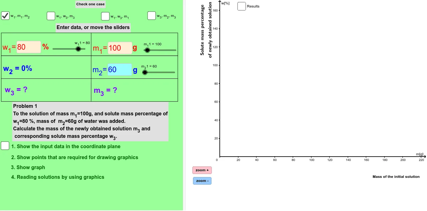
This example demonstrates the graphical solution of mixture problems involving the addition of water, visualizing concentration changes. Core math concepts include ratios, concentration calculations, linear equations, and graphical representation. GeoGebra commands and objects used in construction are highlighted from the summary, such as Line, Intersect, Segment, OrthogonalLine, and Midpoint. Suitable for middle school and above students to understand the integration of graphical methods with mixture problem solving.
GeoGebra Commands & Parameters
Line(B_4, A_4) → iIntersect(i, d) → C_4Textfield(m_11) → inputBoxm_11Textfield(m_21) → inputBoxm_21Textfield(w_11) → inputBoxw_11Textfield(m_32) → inputBoxm_32Line(A_1, C_1) → bIntersect(a, b) → B_1Segment(E_1, C_1) → b_1Segment(C_1, F_1) → c_1Segment(D_1, B_1) → a_1Segment(B_1, G_1) → d_1Segment(A_1, C_1) → g_1Line(A_2, C_2) → pOrthogonalLine(G_2, yAxis) → qIntersect(q, p) → B_2Segment(A_2, C_2) → g_2Segment(G_2, B_2) → d_2Segment(B_2, D_2) → a_2Segment(C_2, E_2) → b_2Line(A_3, B_3) → cSegment(C_2, F_2) → c_2Line(A_3, B_3) → fOrthogonalLine(F_3, yAxis) → gIntersect(g, f) → C_3Segment(G_3, B_3) → d_3Segment(D_3, B_3) → a_3Segment(E_3, C_3) → b_3Segment(C_3, F_3) → c_3Segment(G_4, B_4) → d_4Segment(B_4, D_4) → a_4Midpoint(D_2, E_2) → S_2Midpoint(D_3, E_3) → S_3Midpoint(D_4, E_4) → S_4Textfield(w_12) → inputBoxw_12Textfield(w_13) → inputBoxw_13Textfield(w_33) → inputBoxw_33Textfield(m_13) → inputBoxm_13Textfield(w_32) → inputBoxw_32Textfield(w_34) → inputBoxw_34Textfield(m_24) → inputBoxm_14Textfield(m_34) → inputBoxm_34Midpoint(D_1, E_1) → S_1Segment(F_4, C_4) → c_4Segment(E_4, C_4) → b_4VerticalText(Oy) → OyvVerticalText(Oy2) → Oy2vPolygon(A, B, C, D) → poly1, a_5, b_5, c_5, d_5Vector(A, D) → uTranslate(A, u) → A'Translate(B, u) → B'Translate(C, u) → C'Translate(D, u) → D'Polygon(A', B', C', D') → poly1', a', b', c', d'Translate(A, Vector[(2 * u)]) → A'_1Translate(B, Vector[(2 * u)]) → B'_1Translate(C, Vector[(2 * u)]) → C'_1Translate(D, Vector[(2 * u)]) → D'_1Polygon(A'_1, B'_1, C'_1, D'_1) → poly1'_1, a'_1, b'_1, c'_1, d'_1Point(a_5) → EPoint(c'_1) → FSegment(E, F) → eSegment(A_3, C_3) → g_3Ray(F_3, C_3) → hSegment(A_4, C_4) → g_4Ray(E_4, C_4) → j