
Mixing Two Solutions - Percentage Dynamic Demonstration
Loading the math board and drawing, please wait…
In collections
Chemistry2
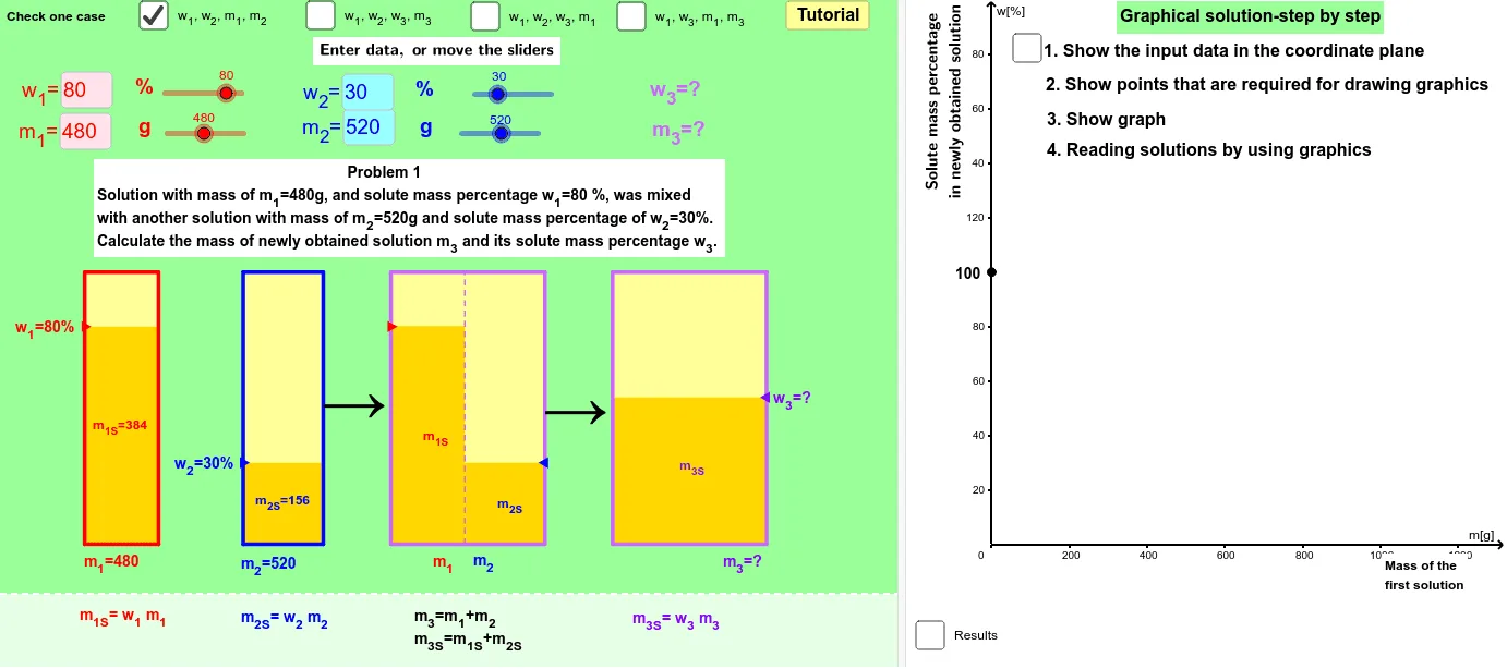
This GeoGebra example dynamically demonstrates the percentage change when mixing two solutions of different concentrations. It visualizes the mathematical modeling of mixture problems, involving core concepts such as ratios, percentages, linear relationships, and function graphs. The construction uses commands like OrthogonalLine, Line, Intersect, Sequence, KeepIf, Element, IndexOf, Textfield, Segment, Midpoint, VerticalText, Min, Max, Polygon, and Ray to build an interactive interface with sliders and live text updates. Suitable for middle and high school students, it aids in understanding proportional reasoning and can be used in mathematics or interdisciplinary chemistry lessons to make abstract mixture problems tangible.
GeoGebra Commands & Parameters
OrthogonalLine(G_2, l) → qLine(A_2, C_2) → pIntersect(q, p) → B_2Sequence((100 * n), n, 0, 200) → list1Line(A_3, B_3) → fIntersect(c, f) → C_3KeepIf(0 < x ≤ 100, list21) → list31Element(list31, 1) → elem1IndexOf(elem1, list21) → index1Element(list1, index1) → scaleLine(A_1, C_1) → bIntersect(a, b) → B_1Line(B_4, C_4) → iIntersect(l, i) → A_4Textfield(m_{11}) → inputBoxm11Textfield(m_{21}) → inputBoxm21Textfield(w_{21}) → inputBoxw21Textfield(w_{11}) → inputBoxw11Textfield(m_{32}) → inputBoxm32Segment(E_1, C_1) → b_1Segment(C_1, F_1) → c_1Segment(D_1, B_1) → a_1Segment(B_1, G_1) → d_1Segment(G_2, B_2) → d_2Segment(B_2, D_2) → a_2Segment(C_2, E_2) → b_2Segment(C_2, F_2) → c_2Segment(G_3, B_3) → d_3Segment(D_3, B_3) → a_3Segment(G_4, B_4) → d_4Segment(B_4, D_4) → a_4Segment(F_4, C_4) → c_4Segment(C_4, E_4) → b_4Segment(A_4, C_4) → g_4Midpoint(D_2, E_2) → S_2Midpoint(D_4, E_4) → S_4Textfield(w_{12}) → inputBoxw12Textfield(w_{22}) → inputBoxw22Textfield(w_{13}) → inputBoxw13Textfield(w_{23}) → inputBoxw23Textfield(w_{33}) → inputBoxw33Textfield(m_{13}) → inputBoxm13Textfield(w_{32}) → inputBoxw32Textfield(w_{14}) → inputBoxw14Textfield(w_{34}) → inputBoxw34Textfield(m_{14}) → inputBoxm14Textfield(m_{34}) → inputBoxm34Midpoint(D_1, E_1) → S_1VerticalText(Oy) → OyvVerticalText(text2) → text3Min(w_{13}, w_{23}) → min3Max(w_{13}, w_{23}) → max3Polygon(H_1, H_2, J_2, J_1) → poly1z1, a_5, b_5, c_5, d_5Polygon(H_1, H_2, I_2, I_1) → poly1b1, d, e, j, kMidpoint(D_3, E_3) → S_3Ray(F_3, C_3) → hPolygon(H_3, H_4, J_4, J_3) → poly1z2, n_1, o_1, t_5, r_5Polygon(H_3, H_4, I_4, I_3) → poly1b2, n_2, o_2, p_5, q_5Polygon(H_8, H_9, I_9, I_8) → poly1b3, u_5, v_1, w_5, x_1Polygon(H_8, H_9, J_9, J_8) → poly1z3, u_6, v_2, z_1, y_1Segment(F_3, C_3) → c_3Segment(C_3, E_3) → b_3OrthogonalLine(F_2, l) → gPolygon(H_5, H_7, I_7, I_5) → poly1, h_5, h_7, i_7, i_5Polygon(H_5, H_6, J_6, J_5) → poly2, h_1, h_6, j_6, j_5Polygon(H_6, H_7, J_7, J_{61}) → poly3, m, n, t_6, e_1Segment(H_6, I_6) → i_1Segment(A_3, C_3) → j_1Segment(A_1, C_1) → l_1Segment(A_2, C_2) → e_2