
Linear Regression: Drag Points or Input Data to Fit a Line
Loading the math board and drawing, please wait…
In collections
ggbchat #4 July 16 2014
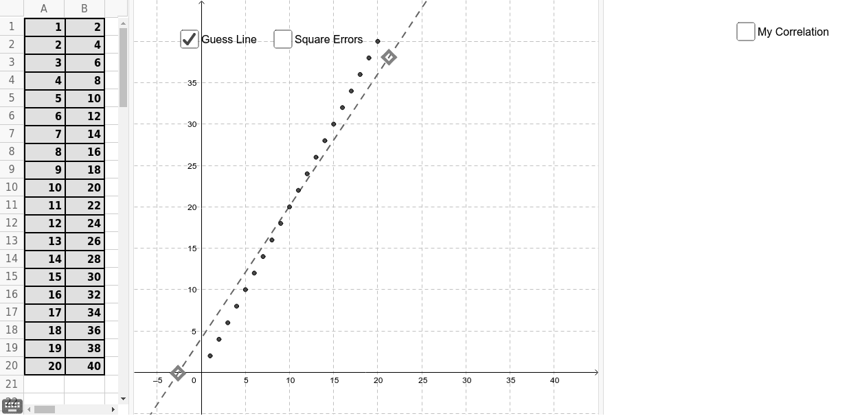
① This example demonstrates how users can define data points by dragging dots or manually entering/modifying them in a spreadsheet, and then observe the fitted linear regression line along with key statistical outputs. ② Core mathematical concepts include least-squares linear regression, residuals, coefficient of determination (R²), sample standard deviation, median, and the equation of the fitted line, as well as intersections between geometric objects. ③ Construction highlights: The GeoGebra command FitLineY computes the regression line, Line draws it, Intersect finds intersection points, Polygon and Vector help visualize data ranges or residual vectors, RSquare and SampleSD calculate statistical measures, Text displays results, Circle may represent confidence intervals or error circles, and data points are managed via spreadsheet objects (A1-A20) and the list list_x. ④ Suitable for high school to undergraduate statistics and data analysis courses, as well as math lab sessions, to deepen understanding of regression analysis and its parameters.
GeoGebra Commands & Parameters
Line(U, V) → line_{guess}Line(A, x = 0) → aLine(B, x = 0) → bLine(C, x = 0) → cLine(D, x = 0) → dLine(E, x = 0) → eLine(F, x = 0) → fLine(G, x = 0) → gLine(H, x = 0) → hLine(I, x = 0) → iLine(J, x = 0) → jLine(K, x = 0) → kLine(L, x = 0) → lLine(M, x = 0) → mLine(N, x = 0) → nLine(NP, x = 0) → npLine(O, x = 0) → pLine(P, x = 0) → qLine(R, x = 0) → sLine(S, x = 0) → tIntersect(line_{guess}, a) → A'Intersect(line_{guess}, b) → B'Intersect(line_{guess}, c) → C'Intersect(line_{guess}, d) → D'Intersect(line_{guess}, e) → E'Intersect(line_{guess}, f) → F'Intersect(line_{guess}, g) → G'Intersect(line_{guess}, h) → H'Intersect(line_{guess}, i) → I'Intersect(line_{guess}, j) → J'Intersect(line_{guess}, k) → K'Intersect(line_{guess}, l) → L'Intersect(line_{guess}, m) → M'Intersect(line_{guess}, n) → N'Intersect(line_{guess}, np) → NP'Intersect(line_{guess}, p) → O'Intersect(line_{guess}, q) → P'Intersect(line_{guess}, s) → R'Intersect(line_{guess}, t) → S'Line(Q, x = 0) → rIntersect(line_{guess}, r) → Q'Polygon(A', A, 4) → poly1, a_1, b_1, c_1, d_1, T, WPolygon(B', B, 4) → poly2, e_1, f_1, g_1, h_1, Z, A_1Polygon(D', D, 4) → poly3, i_1, j_1, k_1, l_1, B_1, C_1Polygon(E', E, 4) → poly4, m_1, n_1, p_1, q_1, D_1, E_1Polygon(C', C, 4) → poly5, r_1, s_1, t_1, a_2, F_1, G_1Polygon(F', F, 4) → poly6, b_2, c_2, d_2, e_2, H_1, I_1Polygon(G', G, 4) → poly7, f_2, g_2, h_2, i_2, J_1, K_1Polygon(H', H, 4) → poly8, j_2, k_2, l_2, m_2, L_1, M_1Polygon(I', I, 4) → poly9, n_2, p_2, q_2, r_2, N_1, O_1Polygon(J', J, 4) → poly10, s_2, t_2, a_3, b_3, P_1, Q_1Polygon(K', K, 4) → poly11, c_3, d_3, e_3, f_3, R_1, S_1Polygon(L', L, 4) → poly12, g_3, h_3, i_3, j_3, T_1, U_1Polygon(M', M, 4) → poly13, k_3, l_3, m_3, n_3, V_1, W_1Polygon(N', N, 4) → poly14, p_3, q_3, r_3, s_3, Z_1, A_2Polygon(NP', NP, 4) → poly15, t_3, a_4, b_4, c_4, B_2, C_2Polygon(P', P, 4) → poly16, d_4, e_4, f_4, g_4, D_2, E_2Polygon(O', O, 4) → poly17, h_4, i_4, j_4, k_4, F_2, G_2Polygon(Q', Q, 4) → poly18, l_4, m_4, n_4, p_4, H_2, I_2Polygon(R', R, 4) → poly19, q_4, r_4, s_4, t_4, J_2, K_2Polygon(S', S, 4) → poly20, a_5, b_5, c_5, d_5, L_2, M_2Vector((x(A), 0), (x(A), y(A) - y(A'))) → V_AVector((x(B), 0), (x(B), y(B) - y(B'))) → V_BVector((x(C), 0), (x(C), y(C) - y(C'))) → V_CVector((x(D), 0), (x(D), y(D) - y(D'))) → V_DVector((x(E), 0), (x(E), y(E) - y(E'))) → V_EVector((x(F), 0), (x(F), y(F) - y(F'))) → V_FVector((x(G), 0), (x(G), y(G) - y(G'))) → V_GVector((x(H), 0), (x(H), y(H) - y(H'))) → V_HVector((x(I), 0), (x(I), y(I) - y(I'))) → V_IVector((x(J), 0), (x(J), y(J) - y(J'))) → V_JVector((x(K), 0), (x(K), y(K) - y(K'))) → V_KVector((x(L), 0), (x(L), y(L) - y(L'))) → V_LVector((x(M), 0), (x(M), y(M) - y(M'))) → V_MVector((x(N), 0), (x(N), y(N) - y(N'))) → V_NVector((x(NP), 0), (x(NP), y(NP) - y(NP'))) → V_{NP}Vector((x(P), 0), (x(P), y(P) - y(P'))) → V_PVector((x(Q), 0), (x(Q), y(Q) - y(Q'))) → V_QVector((x(R), 0), (x(R), y(R) - y(R'))) → V_RVector((x(O), 0), (x(O), y(O) - y(O'))) → V_OVector((x(S), 0), (x(S), y(S) - y(S'))) → V_SRSquare(data, line_{guess}) → StrengthSampleSD(list_y) → SD_yMedian(list_x) → Median_xVector((Median_x / 2, (SD_y * 2)), (Median_x / 2, (SD_y * 2) + over)) → Vector_{over}Vector((Median_x / 2, (SD_y * 2)), (Median_x / 2, (SD_y * 2) - under)) → Vector_{under}Text(((Strength * 100) * "%"), ((Median_x * 1.425), (SD_y * 1.95))) → text1FitLineY(data) → line_{actual}Circle(((Median_x * 1.5), (2 * SD_y)), (Strength * Max[list_y] / 6)) → g_5Circle(((Median_x * 1.5), (2 * SD_y)), (Strength * Max[list_y] / 6)) → CorrelationCircleCircle(((Median_x * 1.5), (2 * SD_y)), (Strength * Max[list_y] / 6)) → CorrelationCircle_1Circle(((Median_x * 1.5), (2 * SD_y)), (Strength * Max[list_y] / 6)) → f_5
AI Drawing Prompt Reference
Create a scatter plot with data points, each connected by a vertical line to a draggable fitted line, forming residual rectangles. The fitted line is defined by two movable points, and data points can be edited in a table. Display the regression equation, R-squared, sample standard deviation, and other statistics, with residual rectangles in distinct colors.
The prompt above was compiled from the original drawing commands and is for reference only.