
Interpreting a Scatter Plot (LR8-01-CYU2)
Loading the math board and drawing, please wait…
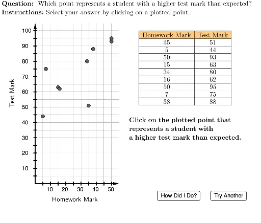
This interactive GeoGebra example is designed to help students practice interpreting scatter plots and understanding relationships between variables. It covers core mathematical concepts such as scatter plots, data distribution, trend analysis, and integrates fractions and binomial distribution as part of the problem contexts. The construction uses a variety of GeoGebra commands including Element, Zip, Sequence, Polygon, Vector, TableText, Text, and Circle to create a dynamic question interface with randomized data points, axis ticks, and feedback markers (correct/incorrect). It is suitable for middle school (e.g., grade 8) statistics and probability lessons, serving as a classroom exercise or self-study tool to develop skills in reading scatter plots and identifying correlations.
GeoGebra Commands & Parameters
Element(questionList, questionListIndex) → situationElement(situationList, situation) → currentSituationZip(A / xInc, A, xVals) → plottedXValsZip(A / yInc, A, yVals) → plottedYValsZip((A, B), A, plottedXVals, B, plottedYVals) → plottedPointsElement(plottedPoints, 8) → HElement(plottedPoints, 5) → EElement(plottedPoints, 2) → BElement(plottedPoints, 1) → AUnicodeToLetter(10007) → xmarkUnicodeToLetter(10003) → cmarkLaTeX((((("\text{" * QUESTION) * "\\") * INSTRUCTIONS) * "}")) → TEXTSequence(Segment[(i, -0.2), (i, 0.2)], i, 1, 10) → xTicksPolygon({(0, 0), (0, 21), (11, 21), (11, 0)}) → viewBoxSequence(i, i, (2 * xInc), 50, (2 * xInc)) → xTickLabelsSequence(i, i, (2 * yInc), 100, (2 * yInc)) → yTickLabelsVector((0, 0), (11, 0)) → xAxisLineVector((0, 0), (0, 21)) → yAxisLineSequence(Segment[(-0.2, i), (0.2, i)], i, 1, 20) → yTicksElement(plottedPoints, 3) → CElement(plottedPoints, 4) → DElement(plottedPoints, 6) → FElement(plottedPoints, 7) → GElement(plottedPoints, 9) → ITableText({Join[{{"\cellcolor{#ffcc80}{\text{Homework Mark}}"}, xVals}], Join[{{"\cellcolor{#ffcc80}{\text{Test Mark}}"}, yVals}]}, "|_vc") → dataRotateText(Text["\text{Test Mark}", (-3, 12), false, true], 90°) → yAxisLabelText("\text{Homework Mark}", (2, -1.5), false, true) → xAxisLabelElement({B, E, A, H}, situation) → correctPointCircle(correctPoint, 0.4) → correctCircleLaTeX((("\text{The point is " * correctPointAdjusted) * ".}")) → feedbackSequence(Text[Element[yTickLabels, i], (-1.75, (2 * i) - 0.25)], i, 1, 20) → yAxisTickLabelsSequence(Text[Element[xTickLabels, i], ((2 * i) - 0.5, -1)], i, 1, 10) → xAxisTickLabelsLaTeX((("\text{Click on the plotted point that\\represents a student with \\" * currentSituation) * ".}")) → currentInstructions
AI Drawing Prompt Reference
Create a scatter plot with labeled axes for 'Homework Mark' on the horizontal axis and 'Test Mark' on the vertical axis, featuring tick marks on both axes. Include multiple randomly plotted data points, with three highlighted in different colors. A table in the lower right corner displays the x and y values for all points. Highlight one correct data point with a circle and label it as 'The point is correct'.
The prompt above was compiled from the original drawing commands and is for reference only.