
Identify Probability Distributions
Loading the math board and drawing, please wait…
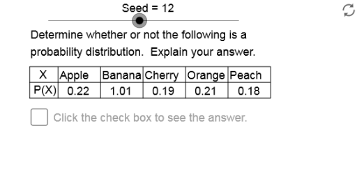
This applet provides several distributions for students to determine if they are probability distributions. Key mathematical concepts include probability and statistics. Using GeoGebra commands such as Sequence, Element, Sum, Mod, If, Sort, and Segment, students can visually understand the characteristics of probability distributions. Suitable for high school and above students learning probability and statistics.
GeoGebra Commands & Parameters
Sequence(Mod[3 + (8 * k), 23], k, 1, 24) → OpSqElement(OpSq, Seed) → OptSequence(Mod[Seed + (Opt * k), Sz1] - round(Sz1 / 2), k, 1, Sz1) → ErSq1Sequence(round(100 / Sz1), k, 1, Sz1) → FrSq0Sequence(Element[FrSq0, k] + Element[ErSq1, k], k, 1, Sz1) → FrSq1Sum(FrSq1) → FrqSmSequence(round((100 * Element[FrSq1, k] / FrqSm)) / 100, k, 1, Sz1) → PrSq1Sequence(Element[PrSq1, k], k, 1, Sz1 - 1) → PrSq2Sum(PrSq2) → PrS2Mod(Opt, 6) → RsltIf(Rslt ≟ 0, Sz1 + 1, Sz1) → Sz2Element(NwPrSq, Rslt + 1) → NwPrbIf(Rslt ≟ 0, Insert[{NwPrb1, NwPrb1A}, PrSq2, Pos], Insert[{NwPrb}, PrSq2, Pos]) → PrSq3Sum(PrSq3) → PrS3Sequence(Mod[2 + (7 * k), 18] + 1, k, 1, 5) → StSqElement(StSq, Mod[Opt, 5] + 1) → St1Element(RtSq, Mod[Opt, 6] + 1) → Rt1If(Rslt ≤ 1, 91, If[Rslt ≟ 2, 97, 107]) → ModNmSequence(Mod[St1 + (k * Rt1), 19] + 2, k, 1, Sz1 - 1) → DvSq1Sort(DvSq1) → DvSq2Element(ErSq2, Mod[Opt, 4] + 1) → ErrSequence(St2 + (k * Rt2), k, 1, Sz2) → TbTR1Segment(TbLT, TbLB) → tblfSegment(TbLT, TbRT) → tbtpSegment(TbLB, TbRB) → tbbtSegment(TbMB, TbMT) → tdlfSegment(TbLM, TbRM) → tbhmElement(CatSq, Mod[Opt, 5] + 1) → TbTR2If(NwPrb < 0, 1, If[NwPrb > 1, 2, If[PrS3 < 1, 3, If[PrS3 > 1, 4, 5]]]) → AnNmElement(AnSq, AnNm) → An0If(Rslt ≟ 3, PrSL, If[Rslt ≟ 4, PrSH, PrS3]) → PrS0Sequence(Mod[Element[OpSq, k], 6], k, 1, 24) → ReSqSum(PrSq1) → PrS4If(Rslt ≟ 0, Insert[{NwPrb1, NwPrb1A}, PrSq2, Pos], Insert[{NwPrb}, PrSq2, Pos]) → PrSq5Sequence(Text[Element[TbTR1, k], (0.5 + (TbCW * k), TbTp - TbCH + 0.1)], k, 1, Sz2) → TbTRTx1Sequence(Text[Element[PrSq3, k], ((TbCW * k) + 0.35, TbTp - (2 * TbCH) + 0.1)], k, 1, Sz2) → TbBRSequence(Segment[(TbDL + (k * TbCW), TbTp), (TbDL + (k * TbCW), TbTp - (2 * TbCH))], k, 1, Sz2) → TbVLSqSequence(Text[Element[TbTR2, k], (0.1 + (TbCW * k), TbTp - TbCH + 0.1)], k, 1, Sz2) → TbTRTx2
AI Drawing Prompt Reference
Create a graph showing multiple probability distributions for educational purposes. Display a series of data points in different colors and shapes, controlled by sliders. Highlight key features of probability distributions, including frequency histograms and probability density curves, along with mathematical calculations. Start by plotting basic data points, then generate frequency and probability distributions, and finally differentiate between distribution types using various colors and line styles, labeling key values.
The prompt above was compiled from the original drawing commands and is for reference only.