
Histogram: Equal Widths and Frequency Distribution
Loading the math board and drawing, please wait…
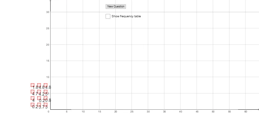
This GeoGebra example demonstrates the construction of a histogram with equal bin widths, illustrating how data is grouped into uniform intervals to show frequency distribution patterns. The core mathematical concepts involved include frequency, relative frequency, class width, piecewise functions, and random sampling in probability statistics. To construct this, the example utilizes several key GeoGebra commands: the Polygon command to draw the bars and boundaries, CountIf for conditional frequency counting, TableText to display the data table, and the Histogram command to generate the plot. The key objects include control vertices A, B, C, D, polygon poly1, and variables a, b, c, d to dynamically update the visual. This example is highly suitable for high school and introductory college-level statistics and probability courses, serving as an interactive tool to understand data binning and histogram generation.
GeoGebra Commands & Parameters
Polygon(A, B, C, D) → poly1, a, b, c, dPolygon(A_1, B_1, C_1, D_1) → poly1_1, a_1, b_1, c_1, d_1Polygon(A_2, B_2, C_2, D_2) → poly1_2, a_2, b_2, c_2, d_2Polygon(A_3, B_3, C_3, D_3) → poly1_3, a_3, b_3, c_3, d_3Polygon(A_4, B_4, C_4, D_4) → poly1_4, a_4, b_4, c_4, d_4Polygon(A_5, B_5, C_5, D_5) → poly1_5, a_5, b_5, c_5, d_5Polygon(A_6, B_6, C_6, D_6) → poly1_6, a_6, b_6, c_6, d_6Polygon(A_7, B_7, C_7, D_7) → poly1_7, a_7, b_7, c_7, d_7Polygon(A_8, B_8, C_8, D_8) → poly1_8, a_8, b_8, c_8, d_8Polygon(A_9, B_9, C_9, D_9) → poly1_9, a_9, b_9, c_9, d_9Polygon(A_{10}, B_{10}, C_{10}, D_{10}) → poly1_{10}, a_{10}, b_{10}, c_{10}, d_{10}Polygon(A_{11}, B_{11}, C_{11}, D_{11}) → poly1_{11}, a_{11}, b_{11}, c_{11}, d_{11}CountIf(B5, list1) → C5CountIf(B6, list1) → C6CountIf(B7, list1) → C7CountIf(B8, list1) → C8CountIf(B9, list1) → C9TableText({{B4, C4}, {B5, C5}, {B6, C6}, {B7, C7}, {B8, C8}, {B9, C9}}, "|_") → text13Histogram({0, 1, 2, 3, 4, 5}, list1) → f
AI Drawing Prompt Reference
Create a histogram with equal‑width bars that visualizes the frequency distribution of a dataset. Use four adjustable anchor points to set the width and position of each bar, and let the bars be drawn sequentially to represent the count of data values falling within each interval. Show a companion table that lists the class intervals together with their corresponding frequencies. The overall layout should clearly display the bars, the interval labels, and the frequency table in a single coherent graphic.
The prompt above was compiled from the original drawing commands and is for reference only.