
Helix with Parametric Equations: Trigonometry-Based 3D Curve Construction
Loading the math board and drawing, please wait…
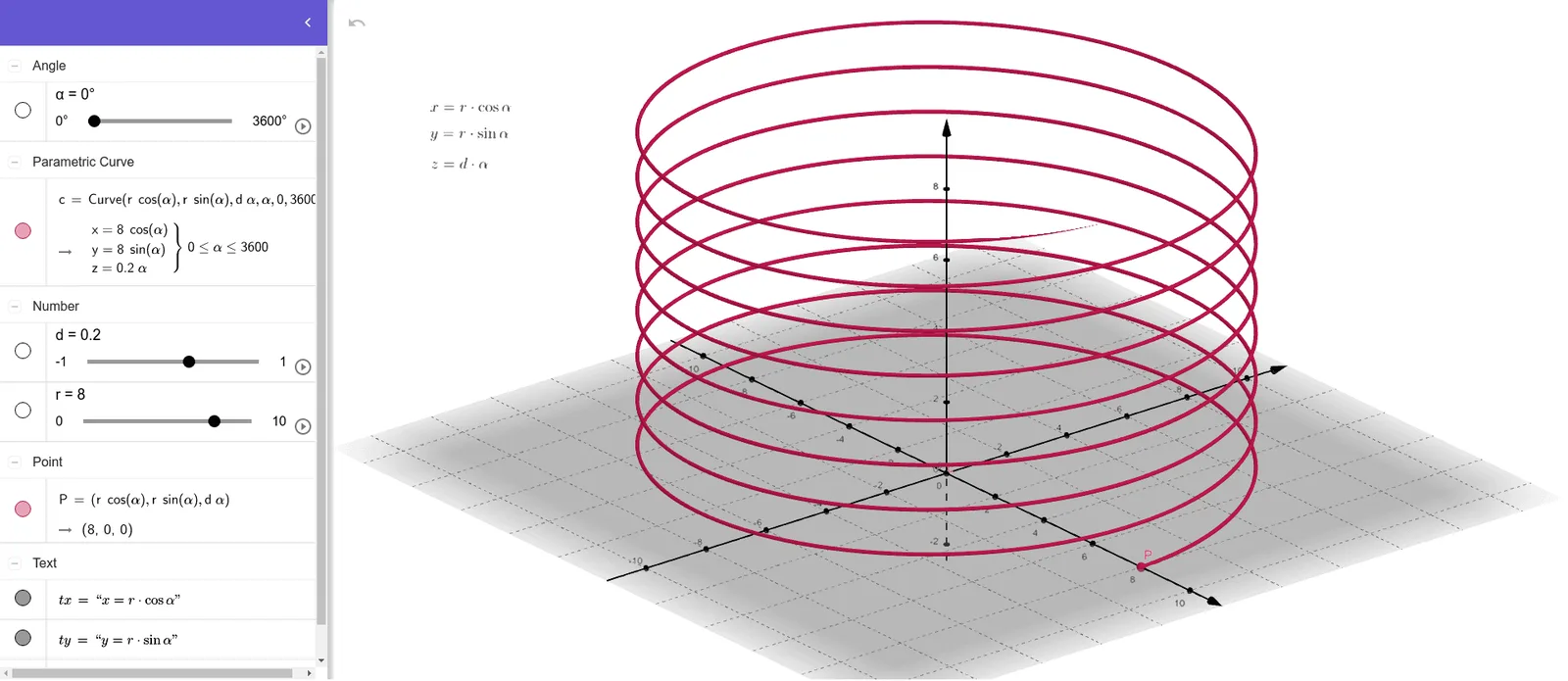
This example demonstrates how to construct and visualize a helix (Helix) in 3D: the curve continuously rises while wrapping around an axis with periodic circular motion. Key concepts include parametric equations, trigonometric functions (sine/cosine to drive the circular projection), and the idea of slope/difference to interpret how the curve changes direction and tangency along its path. Construction-wise, the workflow is based on GeoGebra’s CurveCartesian command to generate a Cartesian parametric curve, using objects α, r, d, P, c, and tx/ty/tz to parameterize radius, height increment, point inputs, and the Cartesian components of the helix. The result is a clear, manipulable model for classroom demonstration or self-study in upper-secondary and early undergraduate levels, covering 3D analytic geometry and trig-based parametric modeling.
GeoGebra Commands & Parameters
CurveCartesian((r * cos(α)), (r * sin(α)), (d * α), α, 0, 3600) → c
AI Drawing Prompt Reference
Draw a 3D helix that continuously rises while wrapping around a central axis with periodic circular motion. The radius is controlled by a parameter, and the height increases linearly with the rotation angle. In a 3D coordinate system, represent the curve using parametric equations: the horizontal projection is a circle (driven by cosine and sine functions), and the vertical component rises uniformly with the angle. Construct the path by first setting the radius and height increment, then generate the spiral, and show its tangent direction to illustrate how the curve changes direction. The graphic should clearly display the helix's periodicity, rising slope, and spatial curvature, suitable for classroom demonstration.
The prompt above was compiled from the original drawing commands and is for reference only.