Self-Intersection Points of a Lissajous Curve via Polyline Approximation

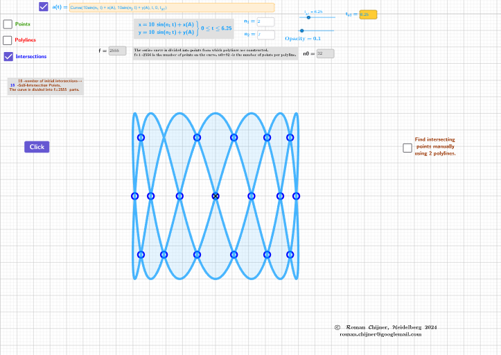
This example demonstrates how to approximate a Lissajous curve with a polyline by sampling the parameter and then locating self-intersection points from intersections of the piecewise-linear segments. The key idea is that a Lissajous curve—built from two sinusoidal components—can cross itself when the frequencies/phase relations produce repeated crossings, and a discrete polyline can reveal where those crossings occur. The core mathematics includes parametric equations, trigonometry (sinusoidal components), and periodic/discrete indexing logic using Mod/Div to control the sampling and segment construction. In GeoGebra, the construction uses Textfield, CurveCartesian to define the curve, Sequence to generate sampled parameters/points, PolyLine to build the polyline approximation, and Element with LaTeX for selecting/labeling relevant objects and displaying results. It also employs Mod and Div to compute step sizes and segment indices, while collecting coordinates (e.g., point lists and polyline segments such as lPoints_y, poly1a/poly2a, and lPoly_y) to identify candidate self-intersections. Suitable for high school to early university students, and useful for teaching parameter curves, discrete numerical approximation, and graph-based reasoning.