
Locus of a Point with Constant Weighted Sum of Squared Distances to N Fixed Poin
Loading the math board and drawing, please wait…
In collections
Besondere Punkte/Special Points
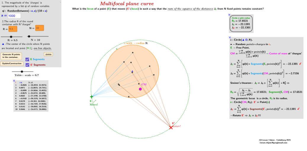
This example visualizes the locus of a moving point in the plane such that the weighted sum of the squared distances from the point to N fixed points remains constant (equal to c). As the parameters vary, the construction reveals the resulting curve(s), highlighting how a global distance constraint to multiple centers translates into a geometric (typically quadratic) locus. The key math concepts are locus geometry, squared-distance constraints, weighted sums, and the underlying coordinate/analytic geometry viewpoint. Construction approach in GeoGebra: use Textfield and Input boxes to set N, c, and weight/scale parameters; generate fixed points via RandomPointIn (e.g., P1, P2, …); employ Circle and Polygon for visual structure; compute and aggregate the constraint using distance terms combined with Sum, while Zip/Flatten help organize the list of terms; create the solution points with Point and Sequence. ScriptListPointsOn_c and ScriptDelete manage the locus point set as c changes, with scale controlling presentation. Suitable for high school through early university learning—especially lessons on analytic geometry, quadratic loci, and parameterized dynamic geometry.
GeoGebra Commands & Parameters
Textfield(a) → InputBox1Circle(D, R) → cSequence(Random[(-a), a] / a / 10, k, 1, N) → qi, {-0.0685, 0.0070999999999999995, -0.0995, -0.0675, 0.05620000000000001, -0.0182, 0.0179, 0.0313, 0.014299999999999998, 0.0646}Flatten(Sequence[{"P_{" + (m) + "}=RandomPointIn[c]", "ShowLabel[P_{" + (m) + "},false]"}, m, 1, N]) → ScriptListPointsOn_cRandomPointIn(c) → P_{1}RandomPointIn(c) → P_{2}Sequence((("Delete[P_{" * m) * "}]"), m, 3, N) → ScriptDeleteTextfield(N) → InputBox4Polygon(Corner[1] + (5, 5), Corner[2] + (-5, 5), Corner[3] + (-5, -5), Corner[4] + (5, -5)) → poly, f, g, h, iTextfield(R) → InputBox2RandomPointIn(c) → P_{3}RandomPointIn(c) → P_{4}RandomPointIn(c) → P_{5}RandomPointIn(c) → P_{6}RandomPointIn(c) → P_{7}RandomPointIn(c) → P_{8}RandomPointIn(c) → P_{9}RandomPointIn(c) → P_{10}Sum(Sequence[(qi(k) * Distance[points(k), E]^(2)), k, 1, N]) → SQSum(Sequence[(qi(k) * Distance[points(k), CM]^(2)), k, 1, N]) → J_0SQCircle(CM, RSQ) → eZip(Segment[E, a], a, points) → segPoint(e) → E'Sum(Sequence[(qi(k) * Distance[points(k), E']^(2)), k, 1, N]) → SQ'Text("$\scalebox{1}{\bf{ " + text14 + " }}$", Bo1, true, true) → text14aText("$\scalebox{" + (LaTeX[scale]) + "}{\bf" + (LaTeX[TableText[{Append["\textcolor{red}{i}", 1…N], Append["\textcolor{blue}{ ±q}", qi], Append["\textcolor{black}{(x,y)}", points]}, "v"]]) + "}$", Bo2, true, true) → text4Text("$\scalebox{1}{\bf{ " + "\ovalbox{\fgcolor{#009900}{\scalebox{0.8}{Circle\; e\; with\; radius}}\\\fgcolor{#009900}{R_0}=" + (LaTeX[RSQ]) + "\\J_\fgcolor{#009900}{E}=" + (LaTeX[SQ]) + "\\ J_{\fgcolor{red}{E'}}=" + (LaTeX[SQ']) + "}" + " }}$", Bo3, true, true) → text2Zip(Segment[E', a], a, points) → seg1
AI Drawing Prompt Reference
Draw a dynamic geometric figure: place N fixed points randomly in the plane, each with a weight. A moving point E satisfies that the weighted sum of squared distances from E to these fixed points equals a constant c. As c varies, the locus of E forms a curve (typically a conic). Show a reference circle whose radius is determined by the weighted sum, and draw segments from E to each fixed point. Use input boxes to adjust N, c, and weights, and a slider for scaling.
The prompt above was compiled from the original drawing commands and is for reference only.