
Geometric Construction of the Levy Lobster Fractal Curve
Loading the math board and drawing, please wait…
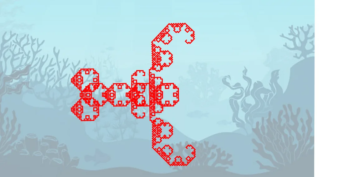
This example demonstrates the step-by-step construction of “Levy's lobster” as a fractal-like curve, showing how a polyline approximation evolves through repeated geometric rules. It highlights key ideas from fractal geometry and parametric/iterated curve sketching, where the final curve emerges from local transformations applied recursively. The construction relies on isosceles-triangle geometry and conditional placement of segments using symmetry operations. In GeoGebra terms, the curve is built by using Join to connect segment endpoints, Sequence to generate the iterative point lists, Take to select the points needed at each step, Translate and Midpoint to position new vertices, and Line to define supporting constraints. Mirror and Rotate are then used to reflect and rotate the current configuration to create the next iteration’s geometry. The objects include named points (e.g., F, A, B, C, D, E, G), multiple point sets (points1…points10), lines (l1…l8 and their transformed counterparts), and segments (segment1…segment7), which together encode the direction changes and connectivity that drive the fractal iteration. Suitable for high school to early university learners for fractal/geometry visualization, GeoGebra-based construction exercises, and discussions of iterative methods.
GeoGebra Commands & Parameters
Join({paral[A, B], {B}}) → points1Join({Join[Sequence[paral[Element[points1, k], Element[points1, k + 1]], k, 1, 2]], {B}}) → points2Join({Join[Sequence[paral[Element[points2, k], Element[points2, k + 1]], k, 1, 4]], {B}}) → points3Join({Join[Sequence[paral[Element[points3, k], Element[points3, k + 1]], k, 1, 8]], {B}}) → points4Join({Join[Sequence[paral[Element[points4, k], Element[points4, k + 1]], k, 1, 16]], {B}}) → points5Join({Join[Sequence[paral[Element[points5, k], Element[points5, k + 1]], k, 1, 32]], {B}}) → points6Join({Join[Sequence[paral[Element[points6, k], Element[points6, k + 1]], k, 1, 64]], {B}}) → points7Join({Join[Sequence[paral[Element[points7, k], Element[points7, k + 1]], k, 1, 128]], {B}}) → points8Join({Join[Sequence[paral[Element[points8, k], Element[points8, k + 1]], k, 1, 256]], {B}}) → points9Join({Join[Sequence[paral[Element[points9, k], Element[points9, k + 1]], k, 1, 512]], {B}}) → points10Sequence(Segment[Element[points10, k], Element[points10, k + 1]], k, 1, 1024) → segment10Take(segment10, 321, 400) → l8Translate(l8, Vector[A, A + (1, 2.5)]) → l8'Take(segment10, 1, 320) → l1Take(segment10, 321, 704) → l2Take(segment10, 704, 1024) → l3Take(segment10, 429, 596) → l4Sequence(Translate[l4, Vector[(i * Vector[A, A + (0, 3.25)])]], i, 1, 3) → l4'Translate(Element[l4', 3], Vector[A, A + (2, 1.2)]) → l6Translate(Element[l4', 3], Vector[A, A + (-2, 1.2)]) → l7Midpoint(E, F) → GLine(G, yAxis) → fMirror(l8', f) → l8''Rotate(l1, (-a), D) → l1'Rotate(l3, a, E) → l3'Rotate(B, 90°, A) → B'Midpoint(B, B') → CSequence(Segment[Element[points1, k], Element[points1, k + 1]], k, 1, 2) → segment1Sequence(Segment[Element[points2, k], Element[points2, k + 1]], k, 1, 4) → segment2Sequence(Segment[Element[points3, k], Element[points3, k + 1]], k, 1, 8) → segment3Sequence(Segment[Element[points4, k], Element[points4, k + 1]], k, 1, 16) → segment4Sequence(Segment[Element[points5, k], Element[points5, k + 1]], k, 1, 32) → segment5Sequence(Segment[Element[points6, k], Element[points6, k + 1]], k, 1, 64) → segment6Sequence(Segment[Element[points7, k], Element[points7, k + 1]], k, 1, 128) → segment7Sequence(Segment[Element[points8, k], Element[points8, k + 1]], k, 1, 256) → segment8Sequence(Segment[Element[points9, k], Element[points9, k + 1]], k, 1, 512) → segment9Rotate(l5, 90°, G) → l5'
AI Drawing Prompt Reference
Draw a Levy lobster fractal curve built by iteratively replacing each segment with the two equal sides of an isosceles triangle, producing a polyline that becomes denser at each level. The final curve consists of about a thousand small segments, showing self-similar branching. Select several portions of the curve, then translate, rotate, or mirror them to create auxiliary reference lines, and mark key points such as midpoints, rotation centers, and an axis of symmetry. The overall composition illustrates the recursive geometric construction, emphasizing local transformations and global shape emergence.
The prompt above was compiled from the original drawing commands and is for reference only.