
Dynamic Logarithmic Properties Demonstration
Loading the math board and drawing, please wait…
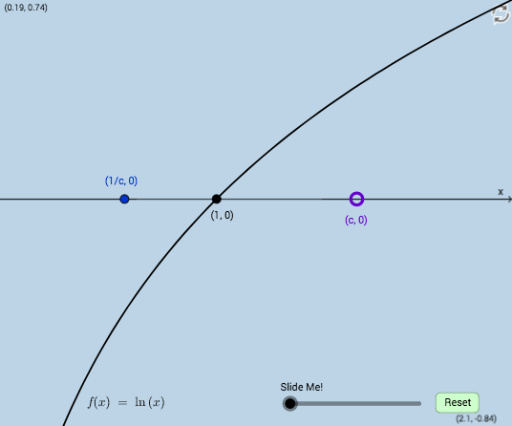
This example dynamically illustrates the reciprocal property of logarithmic functions through interactive geometry, showcasing the geometric characteristics of logarithmic functions. It involves core mathematical concepts such as logarithmic functions, vectors, sequences, and limits in differential calculus. The construction utilizes GeoGebra commands and objects like Textfield, Intersect, Dilate, Segment, Vector, Translate, Rotate, and Distance for dynamic interaction and precise calculations. Suitable for high school and above mathematics learners to understand the properties and geometric applications of logarithmic functions.
GeoGebra Commands & Parameters
Textfield(a) → InputBox1Textfield(f_1) → InputBox2Textfield(f) → InputBox3Intersect(f, h, 1) → EDilate(F, If[0 < d ≤ 1, 1 - d, 0], A) → F'Dilate(A, If[1 < d ≤ 2, 2 - d, 0], B) → A'Segment(A, A') → jDilate(B, If[2 < d ≤ 3, 3 - d, 0], G) → B'Vector(B, B') → uTranslate(A, u) → A'_1Translate(A', u) → A''Segment(A'_1, A'') → j'Rotate(A'_1, If[3 < d ≤ 4, ((-(d - 3)) * π / 2), ((-π)) / 2], F) → HRotate(A'', If[3 < d ≤ 4, ((-(d - 3)) * π / 2), ((-π)) / 2], F) → A'''Segment(H, A''') → j''Rotate(A'_1, If[3 < d ≤ 4, ((d - 3) * π / 2), π / 2], F) → IRotate(A'', If[3 < d ≤ 4, ((d - 3) * π / 2), π / 2], F) → A'''_1Dilate(D, If[4 < d ≤ 5, 5 - d, 0], E) → D'Segment(D, D') → lDilate(A, If[1 < d ≤ 2, 2 - d, 0], C) → A'_2Segment(A, A'_2) → mDilate(A, If[2 < d ≤ 3, 3 - d, 0], R) → C'Vector(C, C') → vIntersect(f, p, 1) → NRotate(F, If[5 < d ≤ 6, ((d - 5) * π / 2), π / 2], F) → F'_1Rotate(F', If[5 < d ≤ 6, ((d - 5) * π / 2), π / 2], F) → F''Dilate(F, If[6 < d ≤ 7, 7 - d, 0], M) → F'_2Vector(F, F'_2) → wTranslate(F'_1, w) → PTranslate(F'', w) → F'''Distance(A, C) → distanceACVector(A, A'_2) → iVector(A, C') → b_1Translate(i, b_1) → i'Dilate(W, If[6 < d ≤ 7, 7 - d, 0], L) → W'Vector(W, W') → w_1Distance(W, L) → distanceWLDilate(T, If[2 < d ≤ 3, 3 - d, 0], U) → T'Vector(T, T') → eDistance(T, U) → distanceTURotate(C, If[3 < d ≤ 4, ((-(d - 3)) * π), (-π)], A) → C'_1Vector(A, C'_1) → qDilate(A, If[4 < d ≤ 5, 5 - d, 0], T) → A'_3Vector(A, A'_3) → u_1Translate(C'_1, u_1) → QVector(A'_3, Q) → v_1
AI Drawing Prompt Reference
Draw a dynamic demonstration of logarithmic functions, including function f and its inverse f_1. Use translation, rotation, and scaling operations to illustrate the geometric properties of logarithmic functions. First, input the function expression, then create the graph of the function and its inverse through translation and rotation. Next, use scaling and rotation to demonstrate the properties of logarithmic functions. Finally, use distance calculations to verify certain geometric relationships.
The prompt above was compiled from the original drawing commands and is for reference only.