
Cube Geometry: Shortest Paths Between Opposite Vertices
Loading the math board and drawing, please wait…
In collections
Cube Geometry
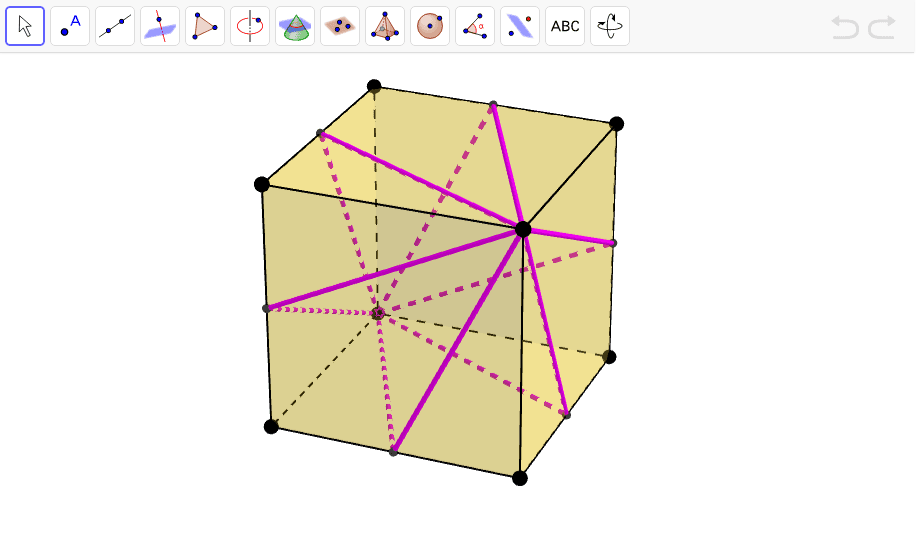
This example demonstrates the 6 shortest paths connecting opposite vertices in a cube. Core math concepts include solid geometry, path optimization, and spatial visualization. It is constructed using GeoGebra commands like Intersect, Point, Cube, Midpoint, and Segment, highlighting key geometric principles. Ideal for high school geometry education and spatial reasoning development.
GeoGebra Commands & Parameters
Intersect(yAxis, zAxis) → APoint(xAxis) → BPoint(Circle[B, Distance[A, B], Segment[A, B]]) → CCube(A, B, C) → a, D, faceCDHG, faceEFGH, edgeAD, edgeAB, edgeBC, edgeCD, edgeAE, edgeDH, edgeEH, edgeEF, E, edgeBF, edgeFG, edgeCG, edgeGH, F, G, H, faceABCD, faceADHE, faceABFE, faceBCGFIntersectMidpoint(edgeAE) → IMidpoint(edgeEH) → JMidpoint(edgeGH) → KMidpoint(edgeCG) → LMidpoint(edgeBC) → MMidpoint(edgeAB) → NSegment(F, J) → cSegment(F, I) → dSegment(F, N) → eSegment(F, M) → fSegment(F, L) → gSegment(F, K) → hSegment(K, D) → iSegment(J, D) → jSegment(I, D) → kSegment(N, D) → lSegment(M, D) → mSegment(L, D) → n