
Cube Cutting Demonstration by Daniel Mentrard
Loading the math board and drawing, please wait…
In collections
Cutting solids by a plane
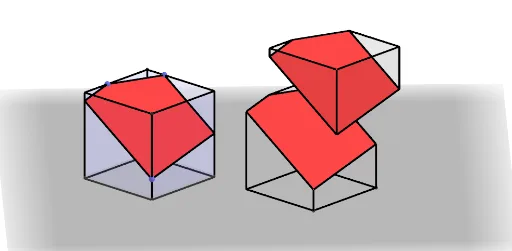
This example demonstrates the geometric forms and spatial relationships after cutting a cube. It involves core mathematical concepts including solid geometry, vector operations, geometric transformations, and optimization problems. GeoGebra commands and objects used in construction include Translate, Segment, Mirror, Polygon, Vector, Point, Line, Intersect, Circle, Cube, Plane, and OrthogonalLine. Suitable for high school students and math enthusiasts to understand spatial geometry and transformation applications.
GeoGebra Commands & Parameters
Translate(O, Vector[(Longueur * u)]) → ASegment(O, A) → dTranslate(O, Vector[(Hauteur / 2^(0.5) * w)]) → CTranslate(O, Vector[(Largeur * v)]) → BSegment(O, B) → eSegment(O, C) → fMirror(A, O) → DMirror(B, O) → EMirror(C, O) → FPolygon(E, A, B, D) → poly1, e_1, a_1, b_1, d_1Vector(O, C) → zTranslate(E, z) → E'Translate(A, z) → A'Translate(B, z) → B'Translate(D, z) → D'Polygon(E', A', B', D') → poly1', e', a', b', d'Mirror(E', O) → E''Mirror(A', O) → A''Mirror(B', O) → B''Mirror(D', O) → D''Polygon(E'', A'', B'', D'') → poly1'', e'', a'', b'', d''Segment(D', A'') → hSegment(B', E'') → iSegment(A', D'') → jSegment(E', B'') → kPoint(k) → HPoint(a') → IPoint(b') → JLine(I, J) → lLine(E', D') → mIntersect(l, m) → Z_2Line(H, Z_2) → nIntersect(n, h) → GLine(A', E') → pIntersect(l, p) → KLine(K, H) → qIntersect(j, q) → LPolygon(L, I, J, G, H) → poly2, l_1, i_1, j_1, g_1, h_1Vector(O, N) → rCircle(N, g, xOyPlane) → sTranslate(N, w) → PLine(N, P) → tIntersect(t, s) → Q, RTranslate(E'', r) → E'''Translate(A'', r) → A'''Translate(B'', r) → B'''Translate(D'', r) → D'''Polygon(E''', A''', B''', D''') → poly1''', e''', a''', b''', d'''Translate(L, r) → L'Translate(I, r) → I'Translate(J, r) → J'Translate(G, r) → G'Translate(H, r) → H'Polygon(L', I', J', G', H') → poly2', l', i', j', g', h'Polygon(H', B''', D''', L') → poly7, h'_4, b'''_1, d'''_1, l'_3Polygon(H', G', A''', B''') → poly8, h'_5, g'_4, a'''_1, b'''_2Line(I', d''') → a1Line(J', e''') → b1Intersect(b1, a1) → SPolygon(L', I', S, E''', D''') → poly9, l'_4, i'_3, s_1, e'''_1, d'''_2Polygon(J', S, I') → poly10, i'_4, j'_4, s_2Point(Circle[D'', Distance[B'', D''], Segment[B'', D'']]) → MCube(B'', D'', M) → a, T, faceMTZW, faceUVWZ, arêteB''T, arêteB''D'', arêteD''M, arêteMT, arêteB''U, arêteTZ, arêteUZ, arêteUV, U, arêteD''V, arêteVW, arêteMW, arêteWZ, V, W, Z, faceB''D''MT, faceB''TZU, faceB''D''VU, faceD''MWVPlane(I', G', H') → p_1OrthogonalLine(N, p_1) → bPoint(b) → A_1Vector(N, A_1) → cTranslate(N, Vector[(g / 2 * c)]) → N'Translate(poly2', Vector[(g / 2 * c)]) → poly2''Translate(G', Vector[(g / 2 * c)]) → G''Translate(H', Vector[(g / 2 * c)]) → H''Translate(I', Vector[(g / 2 * c)]) → I''Translate(L', Vector[(g / 2 * c)]) → L''Translate(J', Vector[(g / 2 * c)]) → J''Line(I'', j'_4) → f_1Line(L'', d'''_2) → k_1Line(H'', b'''_2) → m_1Line(G'', g'_4) → n_1Line(J'', s_1) → q_1Line(I'', k_1) → r_1Line(J'', i'_4) → t_1Intersect(t_1, n_1) → C_1Line(C_1, a'''_1) → c_1Intersect(k_1, f_1) → D_1Intersect(c_1, m_1) → E_1Intersect(m_1, xOyPlane) → F_1Polygon(D_1, E_1, C_1, J'', I'') → poly3, f_2, g_2, h_2, j'', i''Polygon(E_1, H'', L'', D_1) → q1, i_2, h'', l'', j_2Polygon(C_1, G'', H'', E_1) → q2, k_2, g'', l_2, m_2Polygon(J'', C_1, G'') → t1, n_2, p_2, q_2Polygon(D_1, I'', L'') → t2, r_2, t_2, a_2
AI Drawing Prompt Reference
Draw a cube and demonstrate the geometric shapes and spatial relationships after cutting it. Start by establishing the cube's vertices, then use translations, reflections, and rotations to create the cutting plane and the resulting polygons. Finally, determine the intersection lines between the cutting plane and the cube using points and segments to form the cut geometry.
The prompt above was compiled from the original drawing commands and is for reference only.