
Canonical Truncated Snub Cube (V=120) and Its Dual: Edge/Face Coloring
Loading the math board and drawing, please wait…
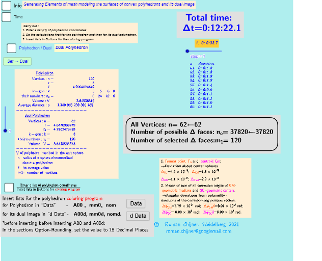
This GeoGebra example visualizes the Canonical Truncated Snub Cube (laevo, V=120) together with its dual image, using systematic edge and face colorings to reveal the correspondence between the two polyhedral structures. It centers on 3D solid geometry and the duality viewpoint for polyhedra, supported by geometric measurements such as distances (via vector/point length computations) and quantitative display of volume-related quantities. Construction-wise, the model uses GeoGebra commands like Text/TableText for labeling, Sequence/IndexOf/First/Element for generating and retrieving structured parameter lists, If for piecewise decisions (e.g., assigning colors or selecting elements), Length for metric computations, Sum for aggregating derived values, and Div for index manipulation. The construction features objects tied to volume metrics (e.g., Volsphere and variants) alongside multiple grouped geometry entities used to drive the coloring of edges and faces. Suitable for advanced high school and early university learners in solid geometry, geometric constructions, and interactive mathematics visualization.
GeoGebra Commands & Parameters
Text("" + p) → txt_pSum(Flatten[Sequence[Append[Sequence[Element[txt_p, i], i, m01(k), m02(k)], " "], k, 1, 5]]) → txtUm1If(bu0, A00, A00d) → A00_0Length(A00_0) → nLength(l2) → läl2Sequence(sgn(Determinant[{Element[A00_0, i1] - Element[A00_0, j], Element[A00_0, i2] - Element[A00_0, j], Element[A00_0, i3] - Element[A00_0, j]}]), j, 1, n) → l01Length(A00d) → zzzSum(Zip[(T * F), T, SysTimeAkt1, F, {1, 1000, 60000, 3600000, 86400000}]) → TimeAbs1Sum(Zip[(T * F), T, SysTimeAkt2, F, {1, 1000, 60000, 3600000, 86400000}]) → TimeAbs2Div(TimeRelab, 3600) → HDiv(TimeRelab - (H * 3600), 60) → MElement(ZwZeit, step) → text10TableText({Append["a duration", Last[ZwZeit, Min[10, Length[ZwZeit]]]]}, "v") → text2cLength(A00) → lm1If(Length[Unique[l01 \ {0}]] ≟ 1, 7, -7) → a7Sum(Zip[(T * F), T, SysTimeAkt0, F, {1, 1000, 60000, 3600000, 86400000}]) → TimeAbs0Div(TimeRelab0, 3600) → H0Div(TimeRelab0 - (H0 * 3600), 60) → M0Text("" + (TimeRelab0 - (H0 * 3600) - (M0 * 60))) → S0aText("" + (TimeRelab - (H * 3600) - (M * 60))) → SIndexOf(".", S) → indexIndexOf(".", S0a) → indexaFirst(S, index + 1) → txtSFirst(S0a, indexa + 1) → txtS0aIf(bu0, " ", "d") → txtbuoMax(Length[A00], Length[A00d]) → maxläElement(A00, 24) → m11TableText({{"\underline{Polyhedron}"}, Append["Vertices: n=", {Length[A00]}], Append["r=", {r}], Append["\bar{r}=", {r_m}], Append["k-gon : k=", mm5a], Append["their\; numbers: n_k=", mm7a], Append["Volume: V=", {Vol_r}], Append["Average\; distance: p=", {txtUm1}]}, "hr ") → text7TableText({{"\underline{dual\;Polyhedron}"}, Append["Vertices: n=", {Length[A00d]}], Append["r=", {r_d}], Append[" \bar{r_d}= ", {r_md}], Append["k-gon : k=", mm5ad], Append["their\; numbers: n_k=", mm7ad], Append["Volume: V=", {Vold_r}]}, "hr ") → text20
AI Drawing Prompt Reference
Draw a canonical truncated snub cube (laevo, with 120 vertices) together with its dual polyhedron, displayed side by side. Both solids are shown in 3D with systematic edge and face colorings to reveal their correspondence. Include labeled vertices, edges, faces, and display metrics such as volume and average distance. Construct the main polyhedron first, then its dual, and finally color the edges and faces and add text labels.
The prompt above was compiled from the original drawing commands and is for reference only.