Constructing the Lemniscate of Bernoulli via Parametric Locus and Intersections

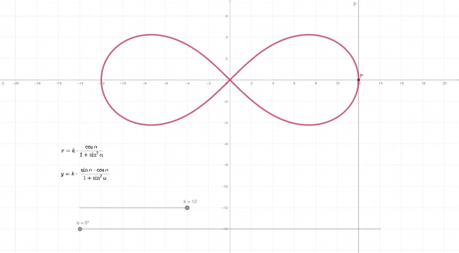
This example demonstrates how to visualize the Lemniscate of Bernoulli: a characteristic two-branch curve meeting at the origin, produced through a parametric, construction-based approach. It highlights key ideas such as locus construction, parametric equations (parametric curves), and the way trigonometric/parameter relations can be encoded into coordinate conditions to drive geometry. In the GeoGebra construction, the workflow is distilled from the provided build summary: the Intersect command is used to determine crucial points (involving objects like k, α, q, p, P, and c), while the Locus command traces the resulting set using computed coordinate components such as tx and ty. The generated geometry makes it easy to study how parameter choices affect the curve’s geometry and symmetry. Suitable for advanced high-school learners and early university students learning coordinate geometry, graphing with GeoGebra, and the locus/parametric-curve method.