
Constructing Polar Curves with Geometric Reflection in GeoGebra
Loading the math board and drawing, please wait…
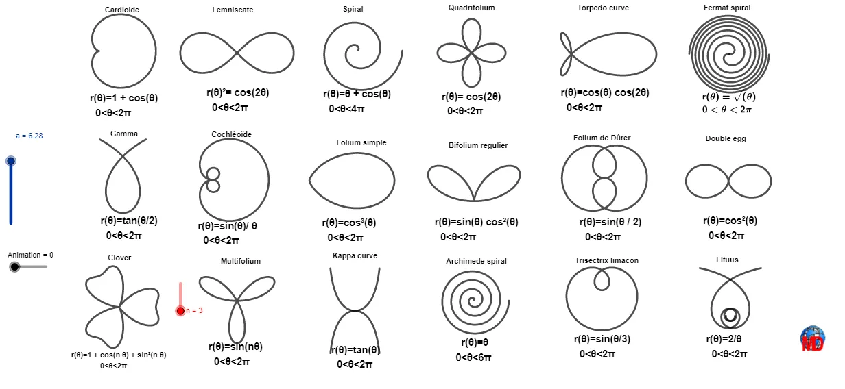
This example demonstrates how polar curves (or equivalent parameter/segmented curve forms) can be generated and visualized on a Cartesian plane using geometric construction and symmetry. It emphasizes key ideas such as polar-curve generation, the relationship between polar/parameter descriptions and Cartesian rendering, and the intuitive role of difference and slope (e.g., secant-line style reasoning). Construction highlights: GeoGebra’s CurveCartesian is used to draw the curve from the constructed data/parameter relations; Line provides reference and secant-like lines to support slope/difference interpretation; and Mirror applies reflection across a specified line to produce mirrored branches, making symmetry in the curve immediately visible. Suitable for secondary school through early university learners for curve sketching, transformation-based modeling, and graphing concepts.
GeoGebra Commands & Parameters
CurveCartesian(A + (1 + cos(θ); θ), θ, 0, a) → a_{1}CurveCartesian(B + (1.5 * (sin((n * θ)); θ)), θ, 0, a) → bCurveCartesian(D + (1.5 * (cos(θ)^(2); θ)), θ, 0, a) → dCurveCartesian(F + (3 * ((cos(θ) * cos((2 * θ))); θ)), θ, 0, a) → fCurveCartesian(G + (2 * (sin(θ) / θ; θ)), θ, (-a), a) → gCurveCartesian(J + (2 * (sqrt(cos((2 * θ))); θ)), θ, 0, a) → jCurveCartesian(M + (3 * (cos(θ)^(3); θ)), θ, 0, a) → kCurveCartesian(N + (5 * ((sin(θ) * cos(θ)^(2)); θ)), θ, 0, a) → lCurveCartesian(O + ((1.5 * sin(θ / 2)); θ), θ, (-a), a) → mCurveCartesian(C + (0.125 * (θ + cos(θ); θ)), θ, 0, (2 * a)) → cCurveCartesian(L + (2 / θ; θ), θ, (-2 * a), -1) → pCurveCartesian(L + (2 / θ; θ), θ, 1, (2 * a)) → qCurveCartesian(K + ((0.05 * θ); θ), θ, 0, (4 * a)) → oCurveCartesian(E + (2 * (tan(θ / 2); θ)), θ, ((-a)) / 3.35, a / 3.35) → eLine(S, T) → rCurveCartesian(H + ((1.2 * cos((2 * θ))); θ), θ, 0, a) → hCurveCartesian(Q + ((0.3 * sqrt(θ)); θ), θ, 0, (3.5 * a)) → uCurveCartesian(Q + ((-0.3 * sqrt(θ)); θ), θ, 0, (3.5 * a)) → tCurveCartesian(R + (tan(θ); θ), θ, ((-a)) / 6, a / 6) → vMirror(v, R) → v'CurveCartesian(I + (0.65 * (1 + cos((n * θ)) + sin((n * θ))^(2); θ)), θ, 0, a) → iCurveCartesian(T + ((1.42 * sin(θ / 3)); θ), θ, 0, (2 * a)) → w
AI Drawing Prompt Reference
On the same Cartesian plane, draw several polar/parameter-style curves to form a curve set. Start by plotting multiple θ-parameterized branches, each built from combinations of sin and cos with varying frequencies, powers, and products, including shifted-center forms, as well as curves involving tan(θ/2) or tan(θ), sqrt(cos(2θ))-type terms, and fractions depending on θ. Add a reference line segment connecting two chosen points to provide a visual slope/secant-like reference. Then mirror the relevant curve component across that reference line to create a symmetric second branch. Finally, overlay additional θ-curves with different amplitudes, shifts, and scaling so the figure shows a coherent family of polar curve shapes.
The prompt above was compiled from the original drawing commands and is for reference only.