
Cone Frustum Demonstration
Loading the math board and drawing, please wait…
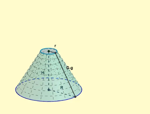
This example demonstrates the geometric construction and visualization of a cone frustum. It involves core mathematical concepts such as solid geometry, volume calculation, and surface area formulas. Key GeoGebra commands used include Circle, Segment, Translate, Cone, and Surface. Suitable for high school students and mathematics enthusiasts learning about three-dimensional geometry and spatial figures.
GeoGebra Commands & Parameters
Circle(C, R, xOyPlane) → cSegment(P, C) → fCircle(P, r, xOyPlane) → dSegment(C, C') → lSegment(P, P') → mSegment(P', C') → nTranslate(P, Vector[(t * u)]) → P'_2Translate(P', Vector[(t * u)]) → P''Segment(P'_2, P'') → m'Cone(C, A, R) → a, e, bSegment(A, C) → iSegment(A, C') → jCone(P, A, r) → k, p, qSegment(A, P) → sSegment(A, P') → f_1Surface(((r + ((1 / H * (H - z)) * (R - r))) * cos(t)), ((r + ((1 / H * (H - z)) * (R - r))) * sin(t)), z, z, 0, H, t, 0, (2 * pi)) → b_1Translate(A, Vector[(t * u)]) → A'_{1}Segment(A'_{1}, P'_2) → g_1Segment(P'', A'_{1}) → h_1Translate(q, Vector[(t * u)]) → q'Translate(p, Vector[(t * u)]) → p'