
Dove Flight Trajectory Demonstration
Loading the math board and drawing, please wait…
In collections
Mat 1 ESO - IESO LA PAZ
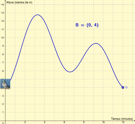
This example demonstrates the mathematical modeling and visualization of a dove's flight trajectory. It involves core math concepts such as secant lines, special points, statistical characteristics, equations, and frequency distribution. Construction highlights include using GeoGebra's Solve command for equation solving, Point for creating points, LaTeX for formula display, Segment for line drawing, and animation (animarpunto) for dynamic simulation. Suitable for high school and above students learning analytical geometry and statistical applications.
GeoGebra Commands & Parameters
Solve(p'(x) = 0) → l1Point(l2) → BLaTeX(B, true, true) → text6Segment((x(B), 0), B) → fSegment((0, y(B)), B) → g
AI Drawing Prompt Reference
Create a coordinate-geometry visualization for a dove flight trajectory concept. Start by locating a key point by solving for where the derivative of the underlying function equals zero. On the coordinate plane, draw two right-angled line segments from this point to the axes: one connects the point to the corresponding position on the x-axis, and the other connects it to the corresponding position on the y-axis. Add a LaTeX-style label showing the point’s coordinate information near the point, so the construction is easy to read.
The prompt above was compiled from the original drawing commands and is for reference only.