
Cobweb Plot Construction
Loading the math board and drawing, please wait…
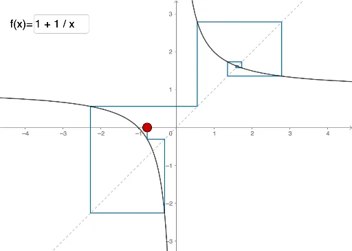
This example demonstrates how to construct a cobweb plot in GeoGebra to analyze the behavior of iterative functions, focusing on convergence and fixed points. Key mathematical concepts include function iteration, dynamical systems, and numerical analysis. The construction utilizes commands like Intersect, Point, Iteration, Sequence, Segment, and Textfield to create the plot dynamically. Suitable for high school and advanced learners exploring calculus and discrete mathematics.
GeoGebra Commands & Parameters
Intersect(f, g, (1.618033990438303, 1.6180339881049803)) → A_1Intersect(f, g, (-0.618033992715713, -0.6180339783672482)) → BPoint(xAxis) → AIteration(f, x(A_1), n) → aSequence(Iteration[f, x(A), i], i, 1, n) → L_1Sequence(Segment[(L_1(i), L_1(i)), (L_1(i), L_1(i + 1))], i, 1, Length[L_1] - 1) → L_2Sequence(Segment[(L_1(i), L_1(i + 1)), (L_1(i + 1), L_1(i + 1))], i, 1, Length[L_1] - 1) → L_3Segment(A, (x(A), f(x(A)))) → hSegment((x(A), f(x(A))), (f(x(A)), f(x(A)))) → iTextfield(f) → InputBox1
AI Drawing Prompt Reference
Draw a cobweb plot showing the iteration of a function. The plot includes a curve and a series of points connected by line segments. Start from a point on the curve, then compute subsequent points through iteration and connect them. Also include an initial point and the function image to illustrate convergence behavior.
The prompt above was compiled from the original drawing commands and is for reference only.