
Binomial and Normal Distribution
Loading the math board and drawing, please wait…
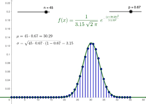
This example demonstrates the graphical representation and relationship between binomial and normal distributions. Key math concepts include probability & statistics, normal distribution properties, binomial distribution models, ellipses, and scatter plots. It utilizes GeoGebra commands like Sequence and Segment in its construction. Suitable for high school students and math enthusiasts studying probability statistics and data analysis.
GeoGebra Commands & Parameters
Sequence(((nCr[n, k] * p^(k)) * (1 - p)^(n - k)), k, 0, n) → sSequence((i, Element[s, i + 1]), i, 0, n) → pointsSequence(Segment[Element[points, i + 1], (i, 0)], i, 0, n) → segmentsSegment(Element[points, k + 1], (k, 0)) → f
AI Drawing Prompt Reference
Create a visual representation showing the relationship between binomial and normal distributions by plotting a set of points for the binomial distribution and connecting them with line segments, then overlaying a normal distribution curve to illustrate the connection between the two distributions, highlighting key concepts in probability and statistics.
The prompt above was compiled from the original drawing commands and is for reference only.