
Butterfly Curve by Daniel Mentrard
Loading the math board and drawing, please wait…
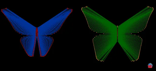
This example demonstrates the generation process of a butterfly curve, involving core concepts of parametric equations and coordinate geometry. Using GeoGebra commands Sequence and objects O, a, l4, l5, l1, b, c, A, l3, l2, l6, l7, l9, B, C, image1, the dynamic changes of the curve can be observed. Suitable for high school mathematics education and learning parametric equations.
GeoGebra Commands & Parameters
Sequence(((((3 / 2 * cos((141 * ((π * k)) / a))^(9)) * (1 - (1 / 2 * sin(((π * k)) / a)))) * (1 - ((1 / 4 * cos((2 * ((π * k)) / a))^(30)) * (1 + cos((32 * ((π * k)) / a))^(20))))) * (1 - (((1 / 2 * sin((2 * ((π * k)) / a))^(30)) * sin((6 * ((π * k)) / a))^(10)) * (1 / 2 + (1 / 2 * sin((18 * ((π * k)) / a))^(20)))))), k, 1, a) → l4Sequence(((cos((2 * ((π * k)) / a)) * cos((141 * ((π * k)) / a))^(2)) * (1 + (((1 / 4 * cos(((π * k)) / a)^(24)) * cos((3 * ((π * k)) / a))^(24)) * cos((21 * ((π * k)) / a))^(24)))), k, 1, a) → l5Sequence((x(O) + Element[l4, i], y(O) + Element[l5, i]), i, 1, Length[l5] - 1) → l1Sequence(((((3 / 2 * cos((141 * ((π * k)) / b))^(9)) * (1 - (1 / 2 * sin(((π * k)) / b)))) * (1 - ((1 / 4 * cos((2 * ((π * k)) / b))^(30)) * (1 + cos((32 * ((π * k)) / b))^(20))))) * (1 - (((1 / 2 * sin((2 * ((π * k)) / b))^(30)) * sin((6 * ((π * k)) / b))^(10)) * (1 / 2 + (1 / 2 * sin((18 * ((π * k)) / b))^(20)))))), k, 1, b) → l3Sequence(Segment[Element[l1, i], Element[l1, i + 1]], i, 1, Length[l1] - 2) → l2Sequence(((cos((2 * ((π * k)) / b)) * cos((141 * ((π * k)) / b))^(2)) * (1 + (((1 / 4 * cos(((π * k)) / b)^(24)) * cos((3 * ((π * k)) / b))^(24)) * cos((21 * ((π * k)) / b))^(24)))), k, 1, b) → l6Sequence((x(A) + Element[l3, i], y(A) + Element[l6, i]), i, 1, Length[l3] - 1) → l7Sequence(Segment[Element[l7, i], Element[l7, i + 1]], i, 1, Length[l7] - 2) → l9
AI Drawing Prompt Reference
Draw a butterfly curve using parametric equations to generate a series of points. Adjust parameters a and b to observe changes in the curve. Start by plotting points O and A, then generate l4 and l3 based on the parametric equations, followed by l1 and l7, and finally connect these points to form l2 and l9, observing the dynamic changes in the curve.
The prompt above was compiled from the original drawing commands and is for reference only.