
Bryan Johnson's Triangle Theorem
Loading the math board and drawing, please wait…
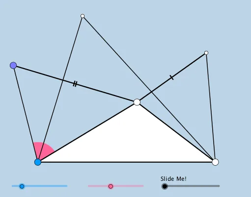
This example demonstrates Bryan Johnson's Triangle Theorem, illustrating the dynamic relationship between triangles and parallelograms. Key mathematical concepts include geometric construction, rotation, angles, vectors, and polygon formation. Construction highlights involve GeoGebra commands such as Segment, Rotate, Angle, Ray, Point, Polygon, Circle, Intersect, Min, CircleSector, Dilate, Vector, and Translate. Suitable for high school and advanced learners to explore geometric proofs and visualizations.
GeoGebra Commands & Parameters
Segment(A, B) → fRotate(B, (a * π / 180), A) → B'Angle(B, A, B') → αRay(A, B') → gPoint(g) → CSegment(B, C) → hSegment(A, C) → iPolygon(A, B, C) → poly1, c, a_1, bRotate(A, If[0 < d ≤ 1, (d * π / 3), π / 3], A) → A'Rotate(C, If[0 < d ≤ 1, (d * π / 3), π / 3], A) → C'Rotate(B, If[0 < d ≤ 1, (d * π / 3), π / 3], C) → B'_1Rotate(C, If[0 < d ≤ 1, (d * π / 3), π / 3], C) → C'_1Segment(A, B) → qRotate(A, If[2 < d ≤ 3, ((d - 2) * π / 3), π / 3], A) → A'_3Rotate(C, (o * π / 180), A) → C'_4Ray(A, C'_4) → tRotate(B, (o * π / 180), C) → B'_3Rotate(B, (o * π / 180), A) → B'_4Ray(C, B'_3) → f_1Ray(A, B'_4) → g_1Point(t) → NCircle(C, (h * e_1)) → h_1Circle(A, (q * e_1)) → k_1Intersect(k_1, g_1, 1) → OIntersect(h_1, f_1) → P,Polygon(A, N, C) → t2, c_2, a_3, n_1Polygon(C, P, B) → t3, b_2, c_3, p_1Polygon(A, O, B) → t4, b_3, a_4, o_1Segment(A, N) → i_1Segment(N, C) → j_1Segment(A, O) → l_1Segment(O, B) → m_1Segment(C, P) → q_1Segment(B, P) → r_1Min(i, i_1) → eCircle(A, (0.2 * e)) → kIntersect(k, i, 1) → DIntersect(k, i_1, 1) → ECircleSector(A, D, E) → pDilate(N, If[0 < d ≤ 1, 1 - d, 0], O) → N'Vector(N, N') → uTranslate(N, u) → N'_1Translate(C, u) → C'_2Segment(N'_1, C'_2) → jDilate(C, If[1 < d ≤ 2, 2 - d, 0], N) → C'_3Vector(C, C'_3) → vTranslate(C, v) → C'_5Translate(P, v) → P'Segment(C'_5, P') → lPolygon(N, C, P, O) → q1, n, c_1, p_2, o_2