
Binomial Probability Problems
Loading the math board and drawing, please wait…
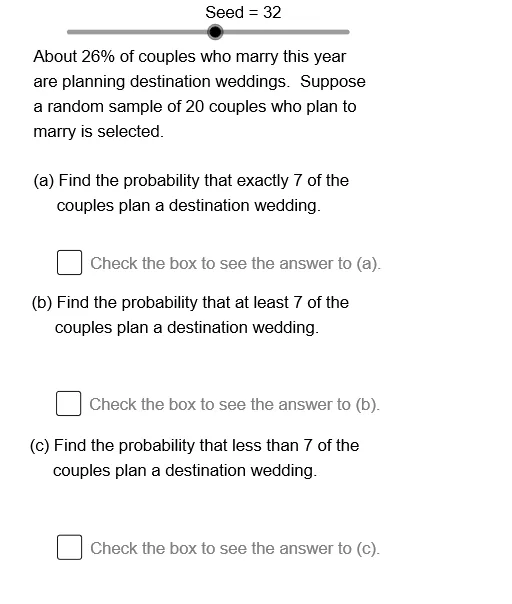
This example demonstrates binomial probability problems. Key mathematical concepts include the calculation of binomial distribution probabilities. Using GeoGebra commands such as Element and Sum, it dynamically shows probability changes. Suitable for high school math education and learning.
GeoGebra Commands & Parameters
Element(StrSq, Mod[Seed, 6] + 1) → StrElement(PrbSq, Mod[Seed, 6] + 1) → ProbElement(RelSq, Mod[Seed + 2, 4] + 1) → RlTrCElement(RelSq, Mod[Seed, 4] + 1) → RlTrBSum(Sequence[((nCr[Size, k] * Prob^(k)) * (1 - Prob)^(Size - k)), k, 0, X - 1]) → CuBiPrLSum(Sequence[((nCr[Size, k] * Prob^(k)) * (1 - Prob)^(Size - k)), k, 0, X]) → CuBiPrEElement(ABSq, Mod[Seed, 4] + 1) → AnBElement(ACSq, Mod[Seed, 4] + 1) → AnCElement(DDSq, Mod[Seed, 6] + 1) → DD0Element(QBSq, Mod[Seed, 6] + 1) → QB0Element(QCSq, Mod[Seed, 6] + 1) → QC0Element(QASq, Mod[Seed, 6] + 1) → QA0
AI Drawing Prompt Reference
Create an educational diagram for binomial probability problems. Include a slider to adjust a random seed, and several text boxes displaying a randomly selected problem statement, a probability value, related condition text, and four answer choices. The main graphic is a dynamic probability distribution chart with the x-axis representing the number of successes and the y-axis representing probability, along with a cumulative probability curve whose left and right endpoints move as the slider changes. Below, display the answer options with the correct one highlighted. The layout should be clear for classroom use.
The prompt above was compiled from the original drawing commands and is for reference only.