
Biased Die Simulation: Probability Distribution and Sample Mean Visualization
Loading the math board and drawing, please wait…
In collections
statistics
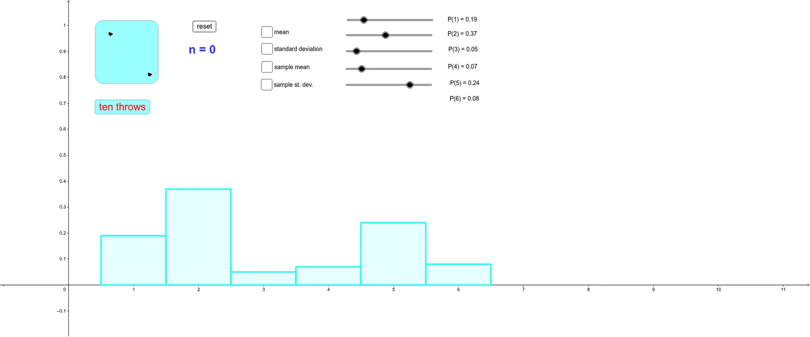
① This GeoGebra example dynamically simulates repeated throws of a biased die, visually showing the frequency distribution of each face and how the sample mean evolves as the number of throws increases. ② Core mathematical concepts include probability distribution, expected value, variance, the law of large numbers, and the difference between sample mean and population mean, involving statistical properties of discrete random variables. ③ Construction highlights: BarChart is used to plot the frequency histogram of each face, Random generates random outcomes, If conditions determine the die face, and AttachCopyToView fixes the view; objects include numeric values a to m, buttons button1 and button2 for throwing and resetting, variable throw for throw count, one to six for face counts, samplemean for the running average, and multiple text objects displaying statistics. ④ Suitable for high school or university probability and statistics courses, this example demonstrates simulation of biased random processes, the relationship between frequency and probability, and the intuitive convergence of sample mean to expectation, serving as an exploratory learning tool.
GeoGebra Commands & Parameters
BarChart(0.5, 6.5, {a, b, c, d, e, f}) → gRandom(0, (100 * a)) → mRandom(1, 100) → tIf(0 < t ≤ (100 * a), 1, If[(100 * a) < t ≤ (100 * (a + b)), 2, If[(100 * (a + b)) < t ≤ (100 * (a + b + c)), 3, If[(100 * (a + b + c)) < t ≤ (100 * (a + b + c + d)), 4, If[(100 * (a + b + c + d)) < t < (100 * (a + b + c + d + e)), 5, 6]]]]) → throwBarChart(0.5, 6.5, {one / n, two / n, three / n, four / n, five / n, six / n}) → oAttachCopyToView(PolyLine[(5.622345707266163, 0.7781013979015848), (5.600015397687656, 0.7762405387700426), (5.622345707266163, 0.7743796796385004), (5.64467601684467, 0.7762405387700426), (5.622345707266163, 0.7781013979015848), (5.600015397687656, 0.7799622570331272), (5.592571961161487, 0.7743796796385004), (5.614902270739995, 0.7706579613754159), (5.629789143792332, 0.7781013979015848), (5.592571961161487, 0.7818231161646694), (5.600015397687656, 0.7762405387700426), (5.622345707266163, 0.7743796796385004), true], 1, (-0.5929237920849864, -0.26025799749899065), (13.616596536371715, 1.2898376590757037), (-571.9999999999993, 638.0000000000001), (1337.0000000000005, -194.99999999999983)) → stroke1AttachCopyToView(PolyLine[(5.622345707266163, 0.7781013979015848), (5.600015397687656, 0.7762405387700426), (5.622345707266163, 0.7743796796385004), (5.64467601684467, 0.7762405387700426), (5.622345707266163, 0.7781013979015848), (5.600015397687656, 0.7799622570331272), (5.592571961161487, 0.7743796796385004), (5.614902270739995, 0.7706579613754159), (5.629789143792332, 0.7781013979015848), (5.592571961161487, 0.7818231161646694), (5.600015397687656, 0.7762405387700426), (5.622345707266163, 0.7743796796385004), true], 1, (-0.5929237920849864, -0.26025799749899065), (13.616596536371715, 1.2898376590757037), (-569.9999999999997, 677.0000000000002), (1339, -155.9999999999999)) → stroke1_1AttachCopyToView(PolyLine[(5.622345707266163, 0.7781013979015848), (5.600015397687656, 0.7762405387700426), (5.622345707266163, 0.7743796796385004), (5.64467601684467, 0.7762405387700426), (5.622345707266163, 0.7781013979015848), (5.600015397687656, 0.7799622570331272), (5.592571961161487, 0.7743796796385004), (5.614902270739995, 0.7706579613754159), (5.629789143792332, 0.7781013979015848), (5.592571961161487, 0.7818231161646694), (5.600015397687656, 0.7762405387700426), (5.622345707266163, 0.7743796796385004), true], 1, (-0.5929237920849864, -0.26025799749899065), (13.616596536371715, 1.2898376590757037), (-479.00000000000006, 734.0000000000003), (1430, -98.99999999999993)) → stroke1_2AttachCopyToView(PolyLine[(5.622345707266163, 0.7781013979015848), (5.600015397687656, 0.7762405387700426), (5.622345707266163, 0.7743796796385004), (5.64467601684467, 0.7762405387700426), (5.622345707266163, 0.7781013979015848), (5.600015397687656, 0.7799622570331272), (5.592571961161487, 0.7743796796385004), (5.614902270739995, 0.7706579613754159), (5.629789143792332, 0.7781013979015848), (5.592571961161487, 0.7818231161646694), (5.600015397687656, 0.7762405387700426), (5.622345707266163, 0.7743796796385004), true], 1, (-0.5929237920849864, -0.26025799749899065), (13.616596536371715, 1.2898376590757037), (-490.99999999999943, 635.0000000000001), (1418, -197.9999999999999)) → stroke1_3AttachCopyToView(PolyLine[(5.622345707266163, 0.7781013979015848), (5.600015397687656, 0.7762405387700426), (5.622345707266163, 0.7743796796385004), (5.64467601684467, 0.7762405387700426), (5.622345707266163, 0.7781013979015848), (5.600015397687656, 0.7799622570331272), (5.592571961161487, 0.7743796796385004), (5.614902270739995, 0.7706579613754159), (5.629789143792332, 0.7781013979015848), (5.592571961161487, 0.7818231161646694), (5.600015397687656, 0.7762405387700426), (5.622345707266163, 0.7743796796385004), true], 1, (-0.5929237920849864, -0.26025799749899065), (13.616596536371715, 1.2898376590757037), (-527.9999999999993, 681.9999999999999), (1381, -150.99999999999991)) → stroke1_4AttachCopyToView(PolyLine[(5.622345707266163, 0.7781013979015848), (5.600015397687656, 0.7762405387700426), (5.622345707266163, 0.7743796796385004), (5.64467601684467, 0.7762405387700426), (5.622345707266163, 0.7781013979015848), (5.600015397687656, 0.7799622570331272), (5.592571961161487, 0.7743796796385004), (5.614902270739995, 0.7706579613754159), (5.629789143792332, 0.7781013979015848), (5.592571961161487, 0.7818231161646694), (5.600015397687656, 0.7762405387700426), (5.622345707266163, 0.7743796796385004), true], 1, (-0.5929237920849864, -0.26025799749899065), (13.616596536371715, 1.2898376590757037), (-568.9999999999998, 728.0000000000001), (1340, -105.00000000000003)) → stroke1_5AttachCopyToView(PolyLine[(5.622345707266163, 0.7781013979015848), (5.600015397687656, 0.7762405387700426), (5.622345707266163, 0.7743796796385004), (5.64467601684467, 0.7762405387700426), (5.622345707266163, 0.7781013979015848), (5.600015397687656, 0.7799622570331272), (5.592571961161487, 0.7743796796385004), (5.614902270739995, 0.7706579613754159), (5.629789143792332, 0.7781013979015848), (5.592571961161487, 0.7818231161646694), (5.600015397687656, 0.7762405387700426), (5.622345707266163, 0.7743796796385004), true], 1, (-0.5929237920849864, -0.26025799749899065), (13.616596536371715, 1.2898376590757037), (-487.9999999999993, 678.0000000000002), (1421, -154.99999999999994)) → stroke1_6
AI Drawing Prompt Reference
Create a dynamic simulation of biased die rolls to visualize the frequency distribution of each face and the evolution of the sample mean as the number of throws increases. Use a bar chart to plot the frequency histogram for each face, generate random outcomes using a random number generator, and determine each face's appearance based on its probability. Plot the trend line of the sample mean and display statistical information such as expected value and variance as the number of throws grows.
The prompt above was compiled from the original drawing commands and is for reference only.