3D Length Visualization with Distributions: Prism Geometry, Slope, and Differenc

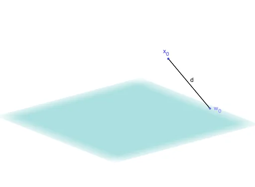
This example uses a 3D prism-based construction to visualize how “length” in three-dimensional space can be represented geometrically and linked to distribution-like behavior as parameters change. Key concepts include solid geometry (constructing a prism and its faces/edges), angle relationships (to encode spatial direction or slicing), and quantitative characterization via differences and slope (together with equation and histogram-style interpretation for discrete quantities). The setup also integrates probability & statistics ideas, aligning geometric modeling with discrete frequency/distribution concepts (e.g., related to a geometric distribution). In GeoGebra, the construction is built using Prism, Segment, and Angle, along with objects such as x0, p, w0–w3, a, x1–x3, and the prism elements face1–face6 and edge1–edge10, plus angle parameters α and β to place and measure the 3D structure. Suitable for high school to early undergraduate learners in solid geometry, mathematical modeling, and probability visualization.