
Zombie Outbreak SIR Model Dynamic Simulation
Loading the math board and drawing, please wait…
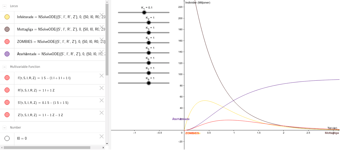
① This GeoGebra example dynamically simulates the spread of a zombie epidemic using the numerical solver NSolveODE, showing how the numbers of susceptible, infected, and recovered individuals change over time. ② The core mathematical concept is a system of ordinary differential equations (SIR model) and its numerical solution, involving transmission and recovery rates, initial conditions, and equilibrium analysis. ③ Construction highlights: the NSolveODE command solves the ODE system with parameters K_1 to K_8 and initial values R0, S0, I0, while objects like Mottagliga (Susceptible), Infekterade (Infected), Återhämtade (Recovered), and ZOMBIES are defined to plot the curves; sliders allow parameter adjustment. ④ Suitable for high school to university courses in mathematical modeling, differential equations, or biomathematics, as well as public health education on epidemic dynamics.
GeoGebra Commands & Parameters
NSolveODE({S', I', R', Z'}, 0, {S0, I0, R0, Z0}, 100) → Mottagliga, Infekterade, Återhämtade, ZOMBIES
AI Drawing Prompt Reference
Create a dynamic simulation graph of a zombie outbreak using the SIR model. The plot should show four time‑dependent curves: susceptible (S), infected (I), recovered (R), and zombies (Z). Include sliders to adjust key parameters such as transmission and recovery rates, and set initial values for each compartment. The graph must clearly illustrate how the numbers of each group evolve, highlighting the epidemic peak, the spread of infection, and the eventual equilibrium where the numbers stabilize. Use smooth lines and a legend to distinguish the curves, and ensure the axes are labeled with time on the horizontal axis and population count on the vertical axis.
The prompt above was compiled from the original drawing commands and is for reference only.