
Jackknife Resampling for Linear Data
Loading the math board and drawing, please wait…
In collections
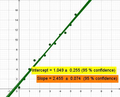
Jackknife resampling to estimate errors in fitted parameters
This example demonstrates how to use Jackknife resampling to estimate the error in parameters fitted to data points, such as the slope of a line. Key mathematical concepts include confidence intervals and standard deviation. GeoGebra commands like Length, Sequence, and Transpose are used to construct the graph. Suitable for high school and above students studying linear regression and statistics.
GeoGebra Commands & Parameters
Length(L) → nSequence(Join[{Take[L, 1, j - 1], Take[L, j + 1, n]}], j, 1, n) → MLSequence(RemoveUndefined[ML(j)], j, 1, n) → ML2Sequence(Fit[ML2(j), {x, 1}], j, 1, n) → RegEqsSequence(Coefficients[RegEqs(k, x)], k, 1, n) → CoeffsTranspose(Coeffs) → CoefficientsSequence(stdev[Coefficients(j)], j, 1, 2) → SdSequence(mean[Coefficients(j)], j, 1, 2) → Av
AI Drawing Prompt Reference
Draw a graph showing the estimation of the slope of a linear regression. The graph should include a set of scatter data points, a fitted line, and an error band representing the standard deviation. The construction order is to first draw the scatter points, then fit the line, and finally add the error band to show the uncertainty of the estimate.
The prompt above was compiled from the original drawing commands and is for reference only.